

Written by Marino San Lorenzo, Consultant
with contribution from Brice-Etienne Toure-Tiglinatienin
This work was produced in 2021 and is based on the module 1 Actuarial Data Scientist training given by the IABE of the same year. This blog post is written for educational purposes.
This article is the first of a series of four articles on this topic:
We intend to raise the awareness on how Data Science can be leveraged on in the context of insurance pricing and how to go from theory to practice, from scripting to deploying your model.
Centuries ago, insurance was introduced to reduce the merchants’ risk of ruining their businesses by losing their cargo to storms or piracy. Getting insured guaranteed some form of compensation if one of these bad events occurs. Thus, merchants were encouraged to take on risks they would otherwise avoid.
Today, the principle is still similar for individuals and companies - they pass their risk onto insurance companies. Insurers need to deal with this uncertainty correctly: the number of claims they will face and what will it cost to settle them. Therefore, insurance companies must assess the risks and define the right prices to charge their clients and maintain the reserve to cover future claims.
Nowadays, insurance companies have a lot of data at their disposal that help them answer the question: “How much on average does my policyholder cost to the insurance undertaking”? Estimating the expected risks purely based on the policyholder’s historical data is often called technical pricing.
Indeed, the role of the Actuary/Data Scientist is to calculate for each policyholder what is the “true” risk of each of its policyholders in its portfolio. This number is crucial. The closer the estimate of Actuary/DS can be (It is impossible to know the true risk that will materialise), the more competitive the insurer can be, proposing lower premiums to attract new policyholders or keep the existing policyholders in its portfolio.
The technical premium is a dominant component of the final insurance premium. [The final premium can be decomposed to technical premium and buffers for handling the policy and marketing (and other costs not directly related to the risk that need to be covered)]. The pricing of an insurance contract puts the Actuary/DS at the forefront of assessing risk. If the model/algorithm the Actuary/DS builds is wrong, the sales of the insurance company can suffer in two ways:
Being as accurate as possible when estimating the real risk of the policyholder is crucial. In this pricing exercise, identifying and quantifying the impact of the main risk factors is a must. Understanding what aggravates or mitigates the risks is also very important to understand for the right pricing of the policyholders. It is also important to explain the risk factors to the brokers who are selling the contracts to make the sales strategy consistent.
As modelling risks involve statistics and programming, we will show one of the technical pricing approaches using Python. This general-purpose language has been gaining popularity over the last decades, even in the actuarial ecosystem where R used to be more dominant.
Before delving into coding and algorithms, we would like to briefly reiterate what we are trying to explain and how is it helping us to understand the risk factors of a given policyholder.
We will illustrate how to price contracts focusing on non-life businesses (home, travel, commercial, motor insurance …). We will show how to measure the pure expectation of the risk for each policyholder for a portfolio of Motor Insurance.
Typically, in Motor Insurance and generally, for Property & Casualty insurance models, the pure premium or risk premium can be broken down into two components: the frequency and the severity.
Source:https://github.com/MarinoSanLorenzo/actuarial_ds/blob/main/blog_post_main.ipynb
It is important to consider the number of claims N as frequencies. Imagine two policyholders. The first had two claims over one year, the second 2 claims over one month. We could think that those two policyholders have the same risk level as they generated the same number of claims. However, the latter generated two claims in one 1month compared to 1 year; the second policyholder is riskier.
Regarding the severity, we need to calculate the expected average loss per claim, given that there was a claim.
Additionally, we strongly assume that the observations of the number of claims are independent but not identically distributed; the same applies to the severity.
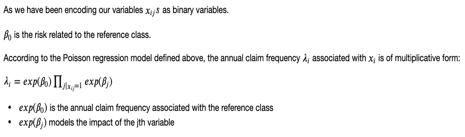
The Poisson regression models the conditional expectation of claims (offset by the exposure of the contract) given the policyholder’s information as follows:
Source:https://github.com/MarinoSanLorenzo/actuarial_ds/blob/main/blog_post_main.ipynb
The same approach will be used to model the severity, except that we won’t account for the exposure and will not consider policies that did not generate claims.
Ultimately, we will fit a Poisson regression model to find the frequency and a Gamma regression model for the severity. Since both the Poisson and Gamma distributions have probability densities from the exponential family, we can leverage the Generalized Linear Models statistical framework to model the relationship between the mean of this distribution and a linear predictor.
Regularisation consists of allowing for a slightly higher bias of our estimator for a larger decrease in the variance of the estimator. We do not want to fit the available data perfectly, but we want the model to perform well on unseen data.
During optimisation and when estimating our parameters, we assign a penalty for the weight of the model parameters as follows:
We want only to keep the parameters that significantly impact our risk. That’s why we force the parameters to go to zero when minimising our loss function. This way, the variables with little added value/information will be discarded.
Another question is how to select the values of the hyperparameters alpha and lambda to regularise our model? [Hyperparameters in contrast to the regular parameters/coefficients (found while fitting the model) are chosen/set by the user before training the algorithm.] This will be addressed in the further section, where we perform a hyperparameter search to know the best hyperparameters to select.
From the two images below, we see that the data is relatively clean - we have no missing values. There are a few categorical variables that we will be encoding and numerical variables that we will be binning for further encoding. This a dataset of 163,657 contracts and 16 variables.
Below is a preview of the dataset:
Source:https://github.com/MarinoSanLorenzo/actuarial_ds/blob/main/blog_post_main.ipynb
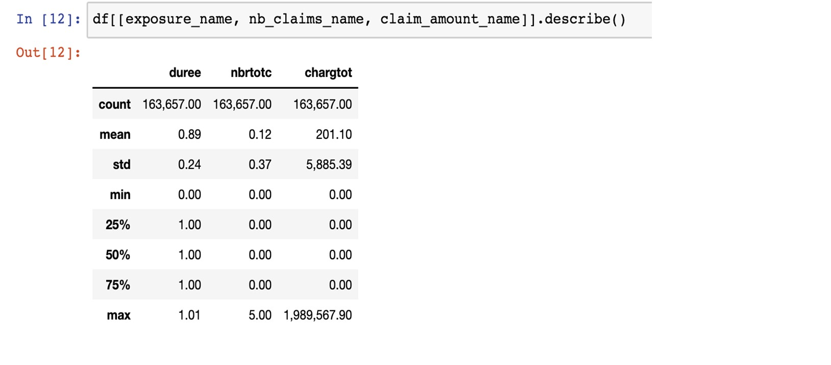
The table below provides some descriptive statistics about the exposure, the number of claims and the claim loss. For the exposure, we can notice that policies are mostly arranged for one year. The minimum is 0. A few policies have this value and can be removed (or not, they have no claim and therefore no impact). The number of claims and the claim loss mostly equal 0. Out of more than 163,650 policies, only around 18,000 have a cost greater than 0 (around 11% of the portfolio). There is one loss claim greater than 500,000, 23 loss claims between 100,000 and 500,000. We decided to cap the maximum loss claim to 500,000.
Source:https://github.com/MarinoSanLorenzo/actuarial_ds/blob/main/blog_post_main.ipynb
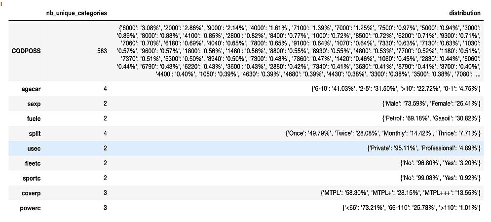
Here below, we see that all categorical variables have a relatively low number of categories except for the CODPOSS variable, which stands for the postal code in Belgium. We do not want such a high dimensional variable. Encoding this variable would add 583 predictors/risk factors to our model, and we want to keep a model as sparse as possible. That’s why later, we will proceed to mean-hot encoding.
Source:https://github.com/MarinoSanLorenzo/actuarial_ds/blob/main/blog_post_main.ipynb
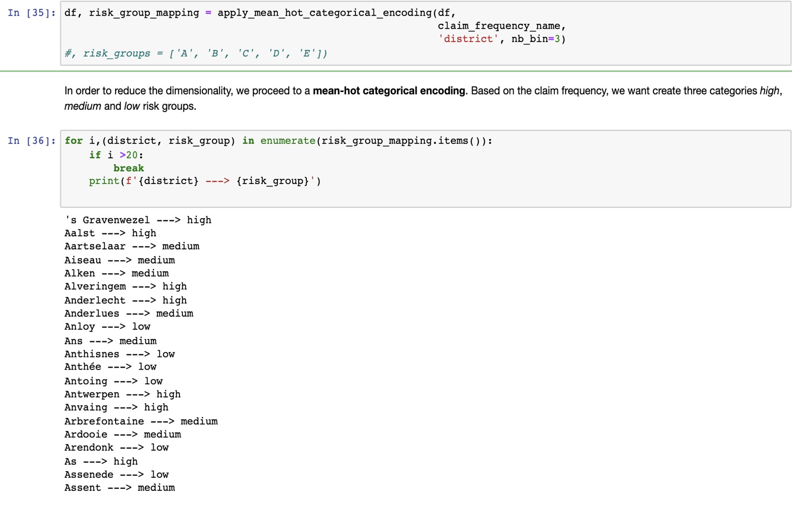
Based on the observed claim frequency, we will divide the CODPOSS categories into 3 groups: {low_risk_district, medium_risk_district, high_risk_district}. This will effectively translate the 583 features from the CODPOSS into 3 categories.
Source:https://github.com/MarinoSanLorenzo/actuarial_ds/blob/main/blog_post_main.ipynb
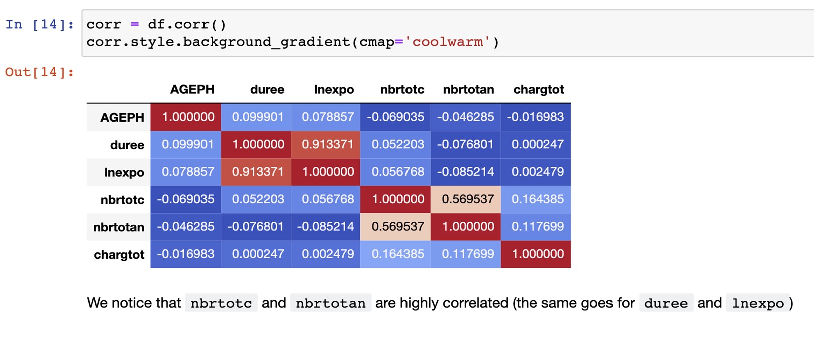
nbrtotc is the number of claims and nbrotan, their yearly claim frequency. Those variables are highly correlated so nbrtotan can’t be used as a predictor simultaneously with nbrtotc.
Source:https://github.com/MarinoSanLorenzo/actuarial_ds/blob/main/blog_post_main.ipynb
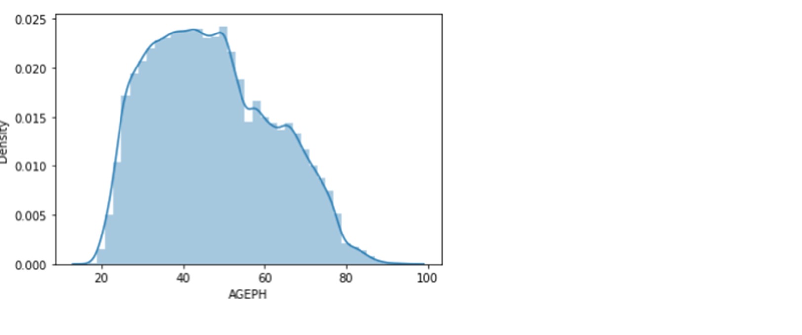
Below is the distribution of the age of policyholders. It varies between 17 and 95 years. The median is 46 years, and the mean is 47 years. The first quartile is 35 years old, and the third is 58 years old. Hence, 50% of the policyholders are between 35 and 58 years.
Let’s also have a look at other categorical variables.
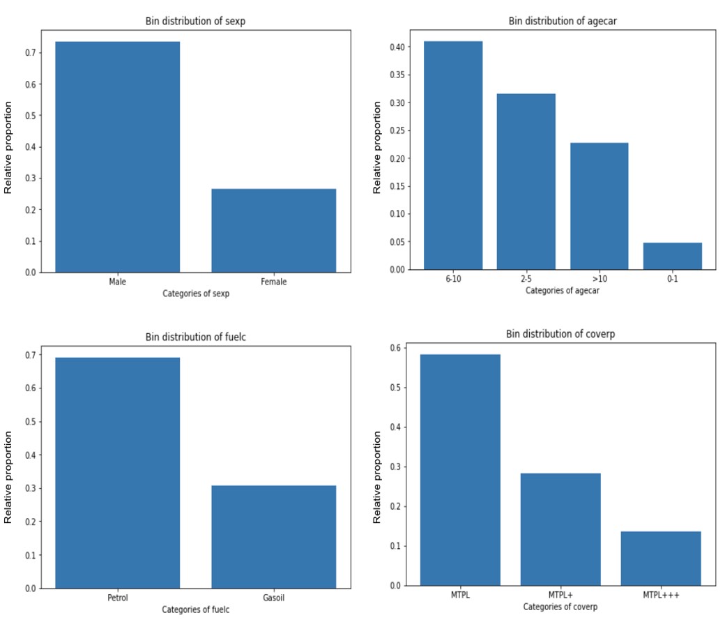
Over 70% of policyholders are males. Around 42% of the cars are between 6 to 10 years old, 32% are between 2 to 5 years, 22% are more than 10 years old, and 4% are between 0 and 1 year old. Almost 70% of these cars use petrol. MPTL is the most bought coverage.
Source:https://github.com/MarinoSanLorenzo/actuarial_ds/blob/main/blog_post_main.ipynb
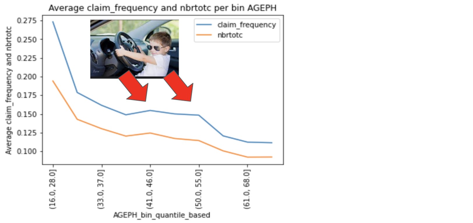
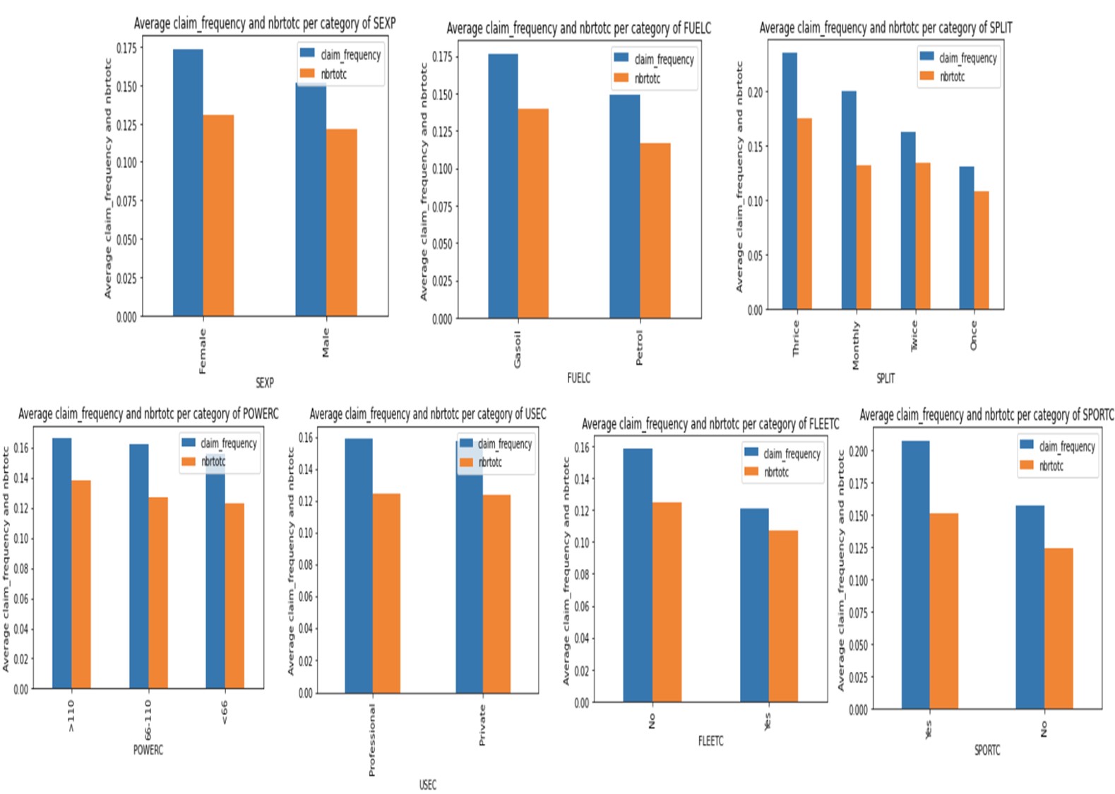
We start with the relationship between the policyholder age and the claim frequency. We plotted the density function of the variables nbrtotc and claim_frequency against the variable AGEPH split into quantile-based groups:
Source:https://github.com/MarinoSanLorenzo/actuarial_ds/blob/main/blog_post_main.ipynb
As the age increases, the densities of claim_frequency and nbrtotc jointly decrease, with a small bump between 41 and 55 years old, which is often when children start to drive their parent’s car. There is a negative relationship between the claim frequency and AGEPH.
Surprisingly, for variable sexp, in this portfolio, the female group is slightly riskier than the male group as the claim frequency for females is slightly higher than the one for males.
Petrol cars seem to be involved in fewer claims than gasoil cars. The policyholders that pay their premium thrice tend to be riskier than those that pay a single premium. Those who pay it monthly seem to be the second riskiest group. The car's usage does not directly impact the claim frequency - both private and professional usage seem to get the same claim frequency.
Policyholders with fleet cars seem to be less frequently involved in claims than those without any. Meantime, policyholders with a sports car tend to get more claims, and it seems that the more power a car has, the more it generates claims, although the difference is narrow. For the variable coverp, the MTPL has the higher claim frequency but the second-highest average claim cost. The cars with MTPL+++ have the highest severity (cars with age between 0 and 1 year have the highest severity).
Source:https://github.com/MarinoSanLorenzo/actuarial_ds/blob/main/blog_post_main.ipynb
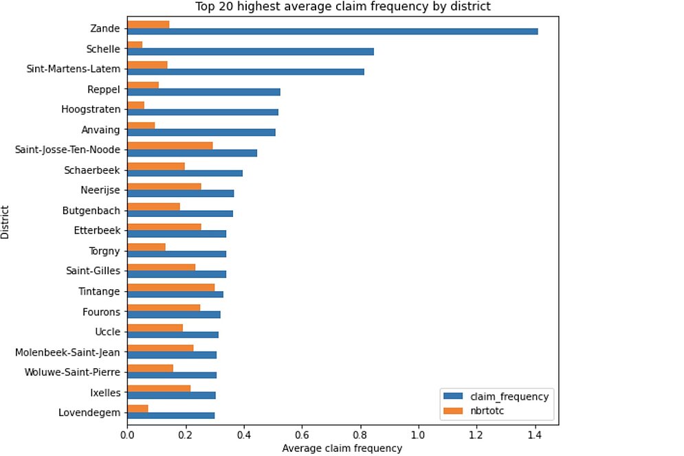
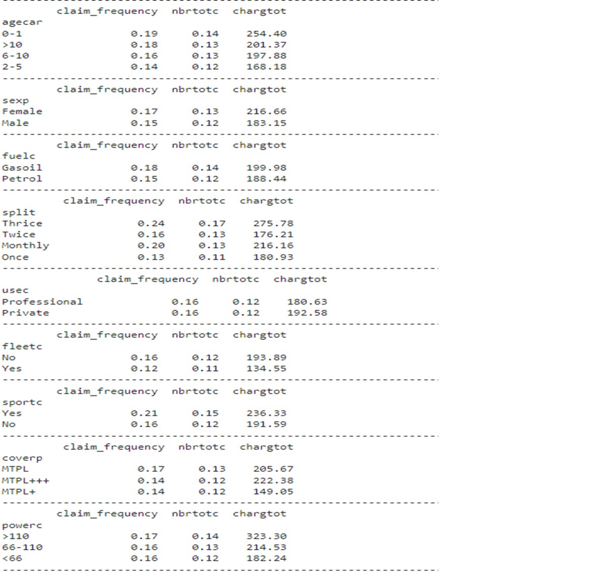
The table below summarizes the average claim frequency, the average number of claims and the average cost of a claim for the different variables.
Source:https://github.com/MarinoSanLorenzo/actuarial_ds/blob/main/blog_post_main.ipynb
The data needs to be numerically encoded for our algorithm/model to read the information we feed it correctly. Let’s start with the numerical variables.
Suppose we had a vector of the age of policyholder as follows with minimum and maximum age going from 0 to 100:
age = (90, 20, 30, 60, 79)
We apply the quantile binning method so that this vector will be transformed in the following matrix:

Source:https://github.com/MarinoSanLorenzo/actuarial_ds/blob/main/blog_post_main.ipynb
Moving on to the categorical variables, we apply a 2-step procedure for encoding the categorical variables:
One-hot encoding works as follows suppose you have a vector of information as follows.
genders = (Male, Female, Female, Female, Male)

Source:https://github.com/MarinoSanLorenzo/actuarial_ds/blob/main/blog_post_main.ipynb
Now, suppose the male group is less risky (as is the case in this dataset), we will decide to take out the gender_male variable from the dataset as it constitutes a reference class.
We will end up with a transformation of our gender vector as follows:

Using this approach, for all xij equal to zero, we get the less risky policyholder's profile and score.
In our dataset example, this is expressed in such a manner:
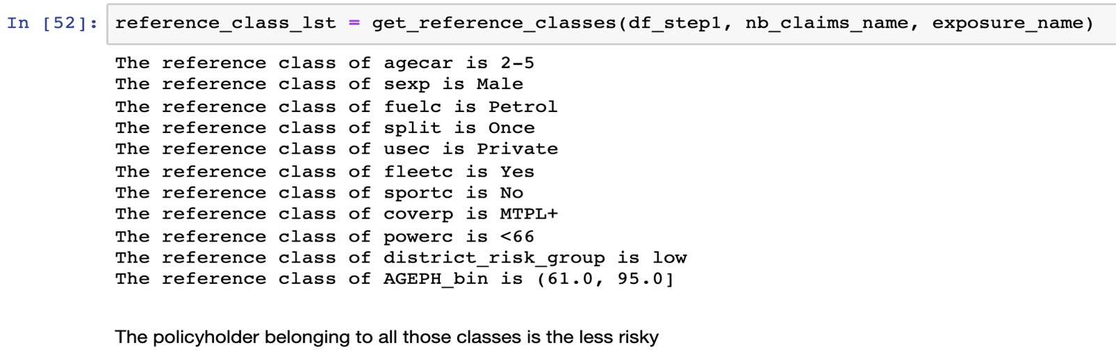
A 61-year-old male policyholder who has a new car, lives in a low-risk district, paid his premium at once and uses his car for private purposes is considered to belong to the least risky reference class.
Source:https://github.com/MarinoSanLorenzo/actuarial_ds/blob/main/blog_post_main.ipynb
To model the conditional expectation of the claim with the exposure as an offset, we use the statsmodel library API.
The first fit with all features returns a result with numerous non-significant features. The p-values, which stand for “what is the probability of observing such data knowing that my parameter is equal to zero”, we observe that usec_Professional, sportc_Yes, coverp_MTPLplusplusplus are not significant.
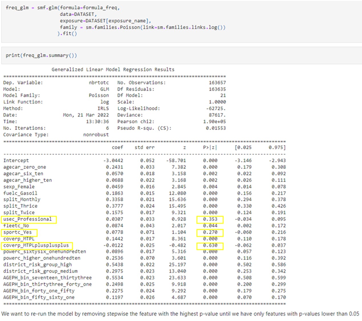
Source:https://github.com/MarinoSanLorenzo/actuarial_ds/blob/main/blog_post_main.ipynb
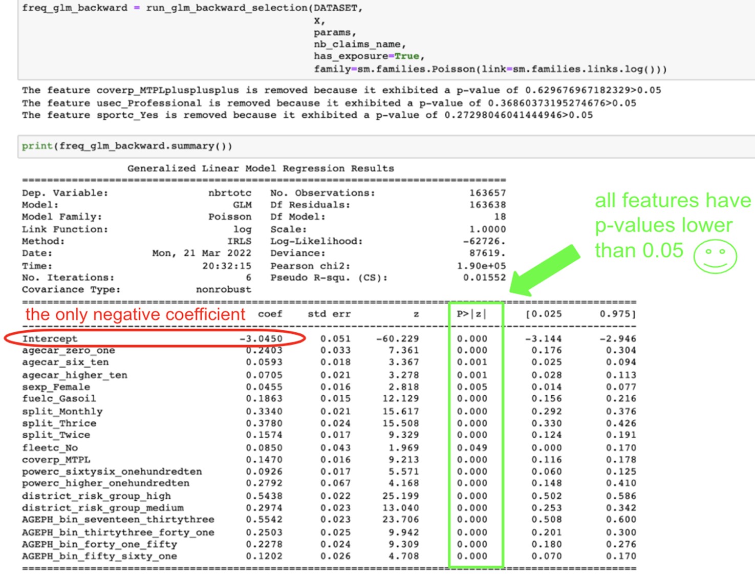
However, how do we know which to remove first and in what order? We probably want to remove first the feature with the highest p-value and then re-fit the model and do this one more time until we only have a significant feature. This is what we did by coding a recursive backward stepwise regression.
run_recursive_backward_stepwise_regression:
Here are the results for the Poisson and Gamma GLM, followed by the features that are discarded
Source:https://github.com/MarinoSanLorenzo/actuarial_ds/blob/main/blog_post_main.ipynb
The starting point for our less risky policyholder is to have an annual claim frequency of exp(-3.0450), which is the exponential of the intercept, which amounts to 0.0475. Living in a high-risk district will increase this frequency by exp(0.5438)=1.722, so 72% so that the annual claim frequency will then become 0.081. We can apply the same reasoning to the other categories.
Notice that because of the way we defined our reference classes, there are no negative values for the coefficients of our features except for the intercept. The intercept is supposed to capture the less risky profile to make sense that no other features decrease the claim frequency. Only the risk factors aggravating the claim frequencies are displayed.
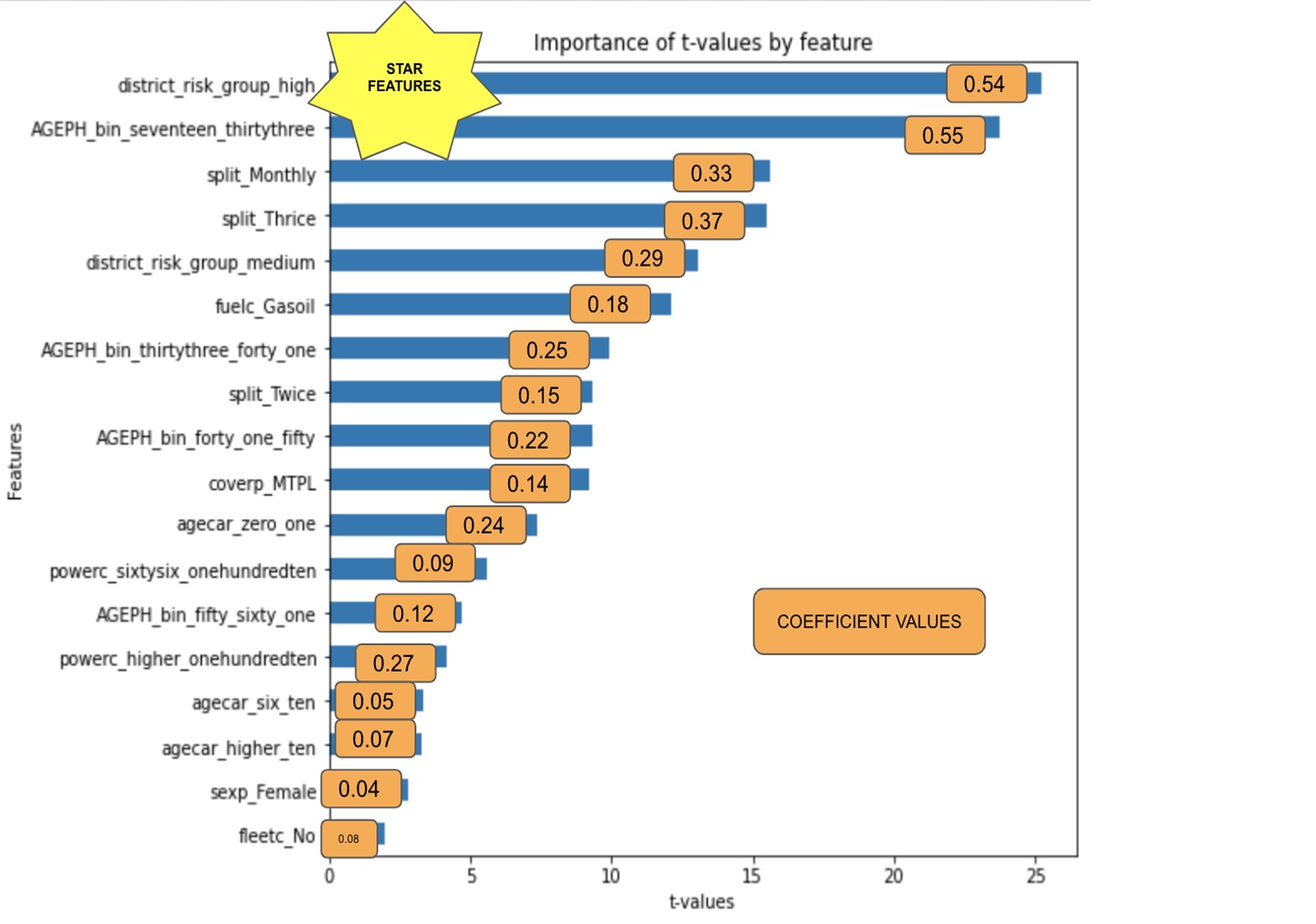
We see that on the top features, the district group, the age and the split variables are the most significant in predicting claims frequencies.
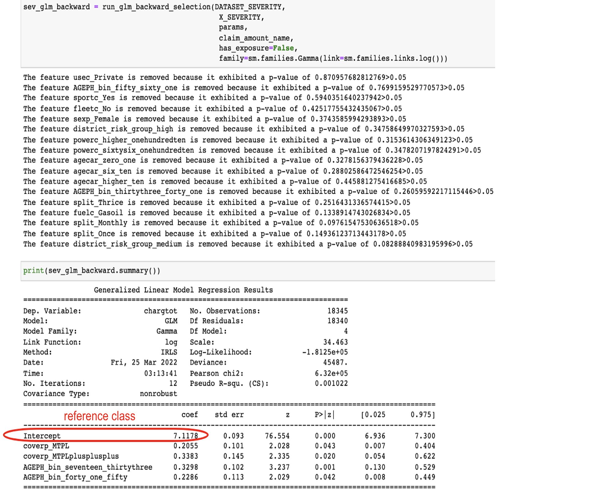
The same can be said about the severity, except that the type of coverage will also be important.
Since we processed our data by setting to zero the less risky profile for both the frequency and severity model, it is easy to know the basic/initial/starting point of the pure premium an insurance will have to charge annually to its less risky potential policyholders.
We multiply the exp(intercep_frequency_model)*exp(intercep_severity_model) = exp(-3.045)*exp(7.1178) = 0.0475*1233.73 = 58.72 whatever unity the claim amount is accounted for. This means that the insurance can’t charge lower than this and more than 1172.97. See below where we generated all possible profiles (11520) and show the riskiest and least risky profile risk premium:
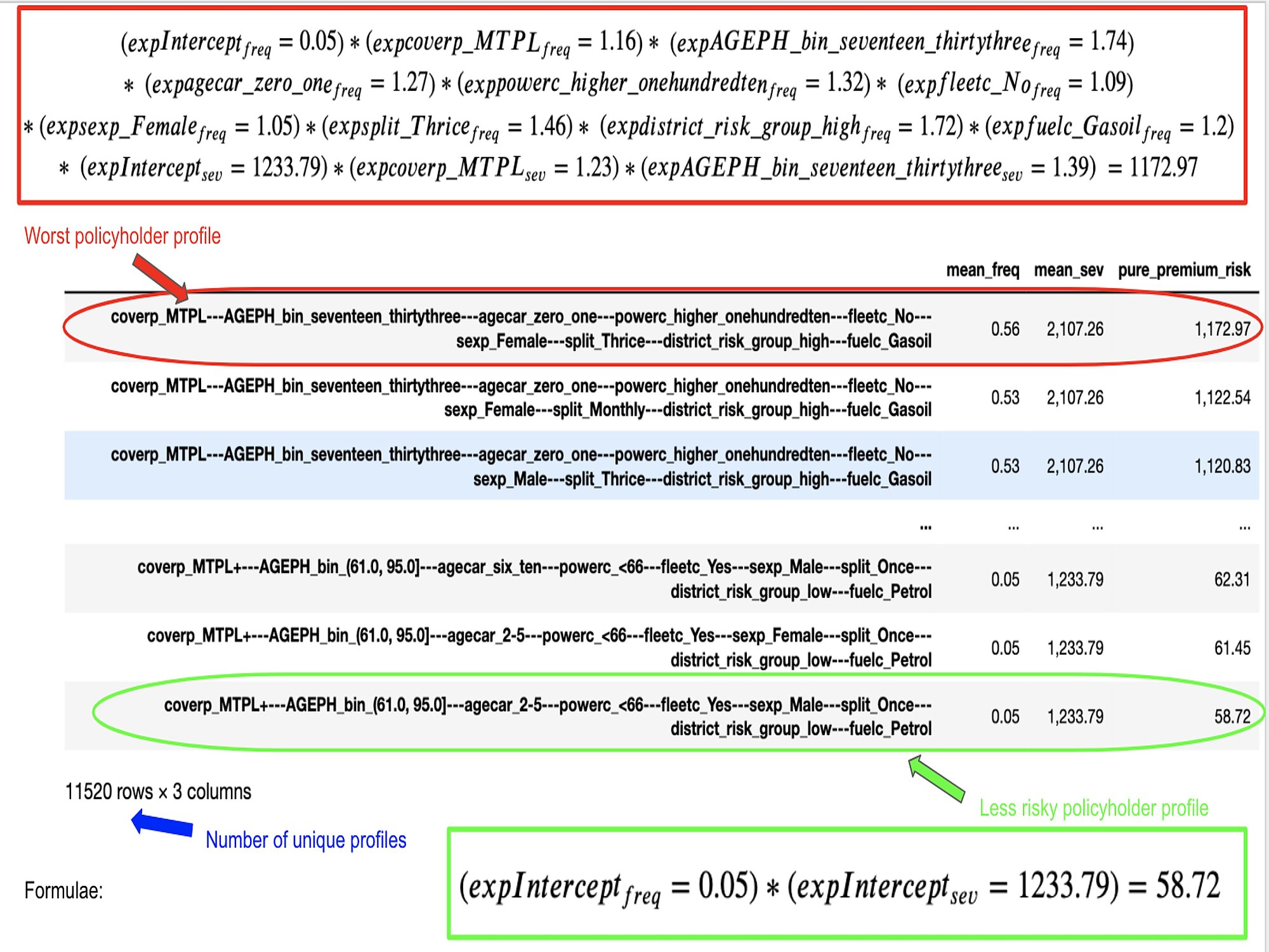
We can store this crude table with the profile names as key and pure_premium_risk as value. This way, when we talk about model serving, our application will instantly return (in O(1)) the risk premium for a given profile.
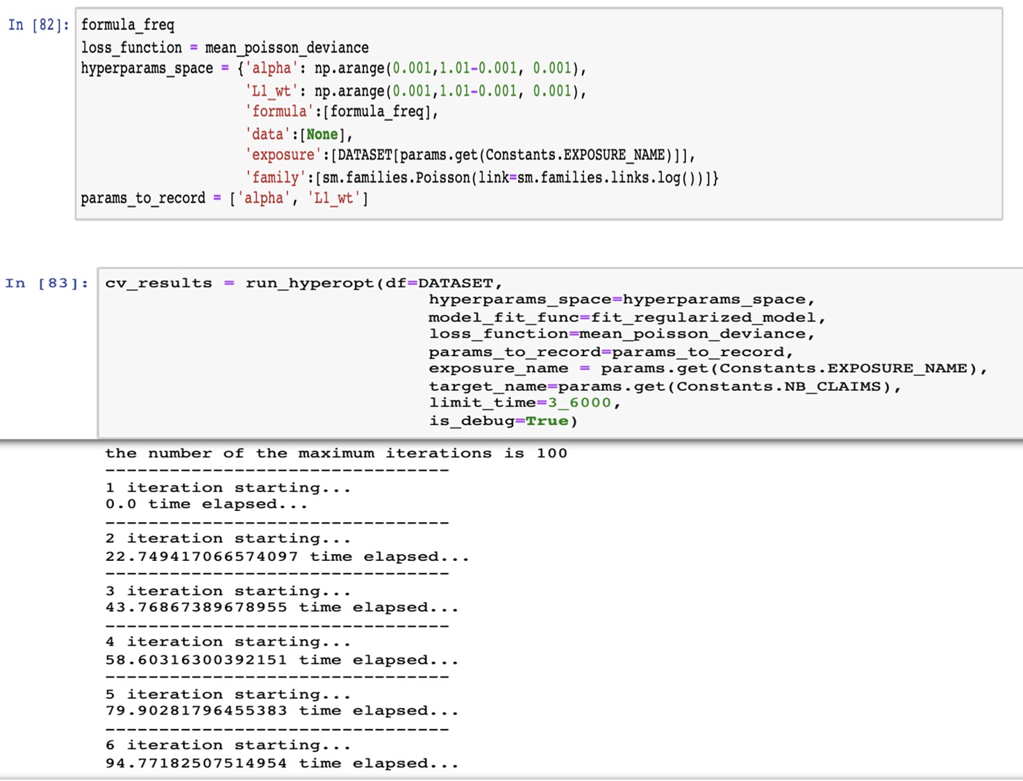
As explained, we want to regularize our model to ensure that this model performs at least as well on unseen data as on training data. We also want to constrain the value of the parameters because we want to select only the most relevant features to work with a sparse model with fewer unnecessary factors to consider.
We perform a random hyperparameter search to find both alpha and lambda.
The algorithm works as follows:
Below, we defined the hyperparameter space with values ranging from 0 to 1 with a step of 0.001.
Then, we set the number of iterations (by default) equals to 100 and to run maximum for 3600s, so 1hour. Afterwards, we go talk to grab a coffee, and we come back to see the results.
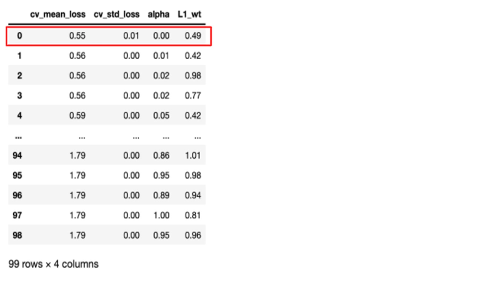
TADAM! Here we have our results ready. We have the mean loss deviance calculated over the k folds along with the standard deviation for each hyperparameter value.
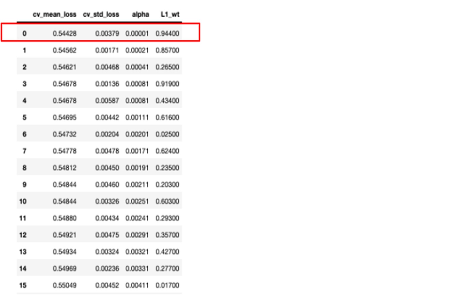
The results are a bit disappointing because we see that the best result is the one with … no regularisation at all with an alpha equal to zero…
Since we can’t go back empty-handed to our manager and tell him that we have been coding hard night and day for nothing, we decide to examine the loss function plotted in 3d with respect to the different hyperparameter values.
When plotting the results, we hope to reach a satisfying minimum by looking around values of alpha very close to zero and with a rather strongly positive value of L1 (area circled in yellow).
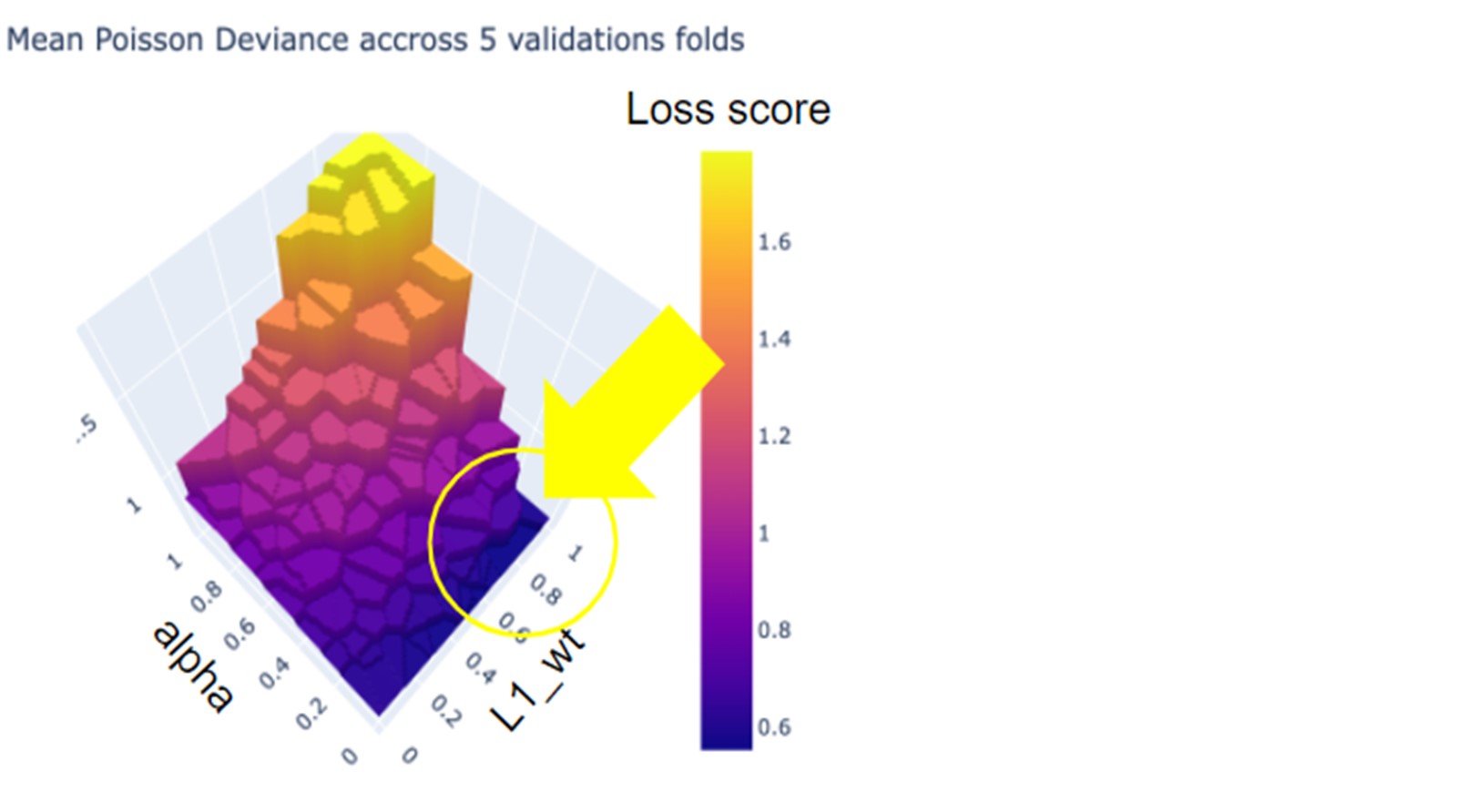
We rerun the search and we reach a slightly lower mean poisson deviance with a small value of alpha=0.00001 and L1_wt=0.944.
When comparing the parameters extracted from the models with and without regularization, we unsurprisingly noticed that the parameters with the largest values come from the unregularized model we fitted in the first place. We can see that AGE_bin_thirtythree_forty_one and coverp_MTPL are features whose coefficients were constrained to zero during the regularisation.
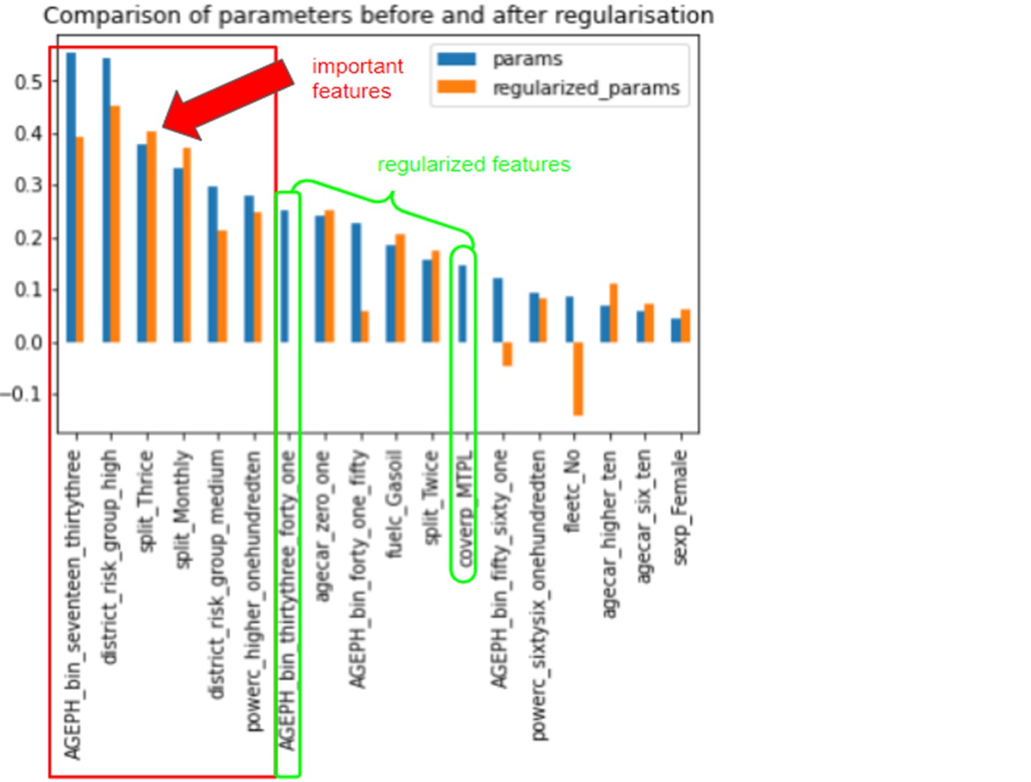
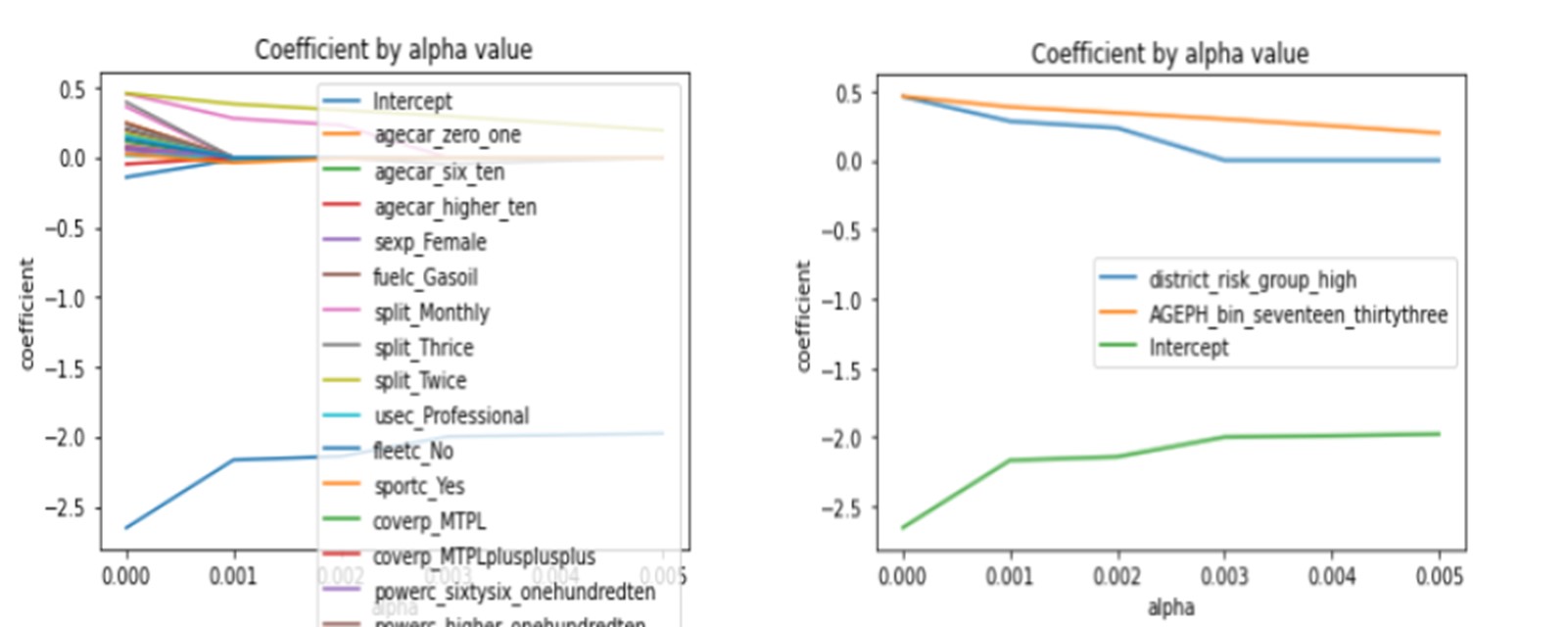
Additionally, when we look more carefully at the variations of the coefficients by features concerning alpha (the regularization parameter), we observe that the two features district_risk_group_high, AGEPH_bin_seventeen_thirtythree and the Intercept (which stands for our reference class) are the parameters converging less rapidly to zero indicating their importance.
Understanding the risk factors and their impacts on the pricing is essential in risk assessment, particularly in a competitive market. In this process, generalised linear models combined with regularisation techniques can be useful. Moreover, GLMs help to understand what impacts your policy's pure premium so the product managers and brokers can effortlessly understand how the model works. In that respect, the GLMs outshine Machine Learning techniques.
By coding our variables as binary and by setting the null vector equal to the reference class corresponding to the less risky profile of the policyholder, we can easily interpret the impact of each feature on the pricing, separately or jointly. By doing so, we can also compare the parameter's features together.
We showed that the most important features for the severity were the following:
For the severity:
For AGEPH, policyholders aged between 17 and 33 generally have a significantly higher claim frequency and severity.
Some additional things could have been done. If we were aiming at improving the model’s performance aside from understanding the risk factors, we could have tried:
We hope that you enjoyed reading our article. If so, please share this article and stay tuned for the next article dealing with Machine Learning in the context of insurance pricing.
Finalyse InsuranceFinalyse offers specialized consulting for insurance and pension sectors, focusing on risk management, actuarial modeling, and regulatory compliance. Their services include Solvency II support, IFRS 17 implementation, and climate risk assessments, ensuring robust frameworks and regulatory alignment for institutions. |

Check out Finalyse Insurance services list that could help your business.
Get to know the people behind our services, feel free to ask them any questions.
Read Finalyse client cases regarding our insurance service offer.
Read Finalyse blog articles regarding our insurance service offer.
Designed to meet regulatory and strategic requirements of the Actuarial and Risk department
Designed to meet regulatory and strategic requirements of the Actuarial and Risk department.
Designed to provide cost-efficient and independent assurance to insurance and reinsurance undertakings
Finalyse BankingFinalyse leverages 35+ years of banking expertise to guide you through regulatory challenges with tailored risk solutions. |

Designed to help your Risk Management (Validation/AI Team) department in complying with EU AI Act regulatory requirements
A tool for banks to validate the implementation of RWA calculations and be better prepared for CRR3 in 2025
In 2027, FRTB will become the European norm for Pillar I market risk. Enhanced reporting requirements will also kick in at the start of the year. Are you on track?
Finalyse ValuationValuing complex products is both costly and demanding, requiring quality data, advanced models, and expert support. Finalyse Valuation Services are tailored to client needs, ensuring transparency and ongoing collaboration. Our experts analyse and reconcile counterparty prices to explain and document any differences. |

Helping clients to reconcile price disputes
Save time reviewing the reports instead of producing them yourself
Helping institutions to cope with reporting-related requirements
Be confident about your derivative values with holistic market data at hand
Finalyse PublicationsDiscover Finalyse writings, written for you by our experienced consultants, read whitepapers, our RegBrief and blog articles to stay ahead of the trends in the Banking, Insurance and Managed Services world |

Finalyse’s take on risk-mitigation techniques and the regulatory requirements that they address
A regularly updated catalogue of key financial policy changes, focusing on risk management, reporting, governance, accounting, and trading
Read Finalyse whitepapers and research materials on trending subjects
About FinalyseOur aim is to support our clients incorporating changes and innovations in valuation, risk and compliance. We share the ambition to contribute to a sustainable and resilient financial system. Facing these extraordinary challenges is what drives us every day. |

Finalyse CareersUnlock your potential with Finalyse: as risk management pioneers with over 35 years of experience, we provide advisory services and empower clients in making informed decisions. Our mission is to support them in adapting to changes and innovations, contributing to a sustainable and resilient financial system. |

Get to know our diverse and multicultural teams, committed to bring new ideas
We combine growing fintech expertise, ownership, and a passion for tailored solutions to make a real impact
Discover our three business lines and the expert teams delivering smart, reliable support