

Written by Marino San Lorenzo, Consultant
with contribution from Brice-Etienne Toure-Tiglinatienin and Hassane Boubacar
Our previous article Actuarial Data Science: Understand your risk factors thanks to Generalized Linear Models and Regularization techniques, showed how traditional statistical techniques such as GLMs can help with assessing the risk factors for a given portfolio and their impacts on the pricing. GLM models are popular due to their straight-forward interpretation.
This article shows how machine learning techniques can boost model performance in terms of prediction accuracy and flexibility. However, these benefits may come with some setbacks: loss of interpretability (our next article will cover this topic) and additional hyperparameters to tune. To illustrate these different methods, we are going to use the French Motor Third-Part Liability dataset. This dataset contains risk features (such as exposure, power, vehicle age, driver age etc.), claim numbers and the corresponding claim amounts for the 413,169 MTPL policies over a one-year period. You can follow the code in the repository here.
When dealing with Machine/Deep Learning models, the performance gains usually come at the cost of model interpretability but also a greater number of hyperparameters to tune. This may add complexity to the training process. We often know which hyperparameters are important but not what values they should have. Similarly to Homer Simpson in front of his nuclear monitoring desk, a data scientist or modeler can feel overwhelmed with the number of buttons/hyperparameters to tweak to get to the optimal results. This article aims at explaining how to find these elusive values.

We outline three main hyperparameter optimisation methods (HOM) to fine-tune algorithms. These HOMs are easy to implement and understand and there are a lot of open-source tools available allowing anyone to try them out. We will now explain the intuition behind these HOMs.
Random search is a method in which random combinations of hyperparameters are selected and used to train a model. The random hyperparameter combination that corresponds to the lowest loss scores is picked. This is similar to when in the previous article we wanted to add regularisation to the GLM model to prevent overfitting; we arbitrarily chose two values for the two parameters alpha and L1_wt and wrote a procedure that:
Finally, we selected “the best hyperparameters”, i.e. the vector/combination of values which rendered the lowest loss score on the test dataset (see section Adding more regularization for details).
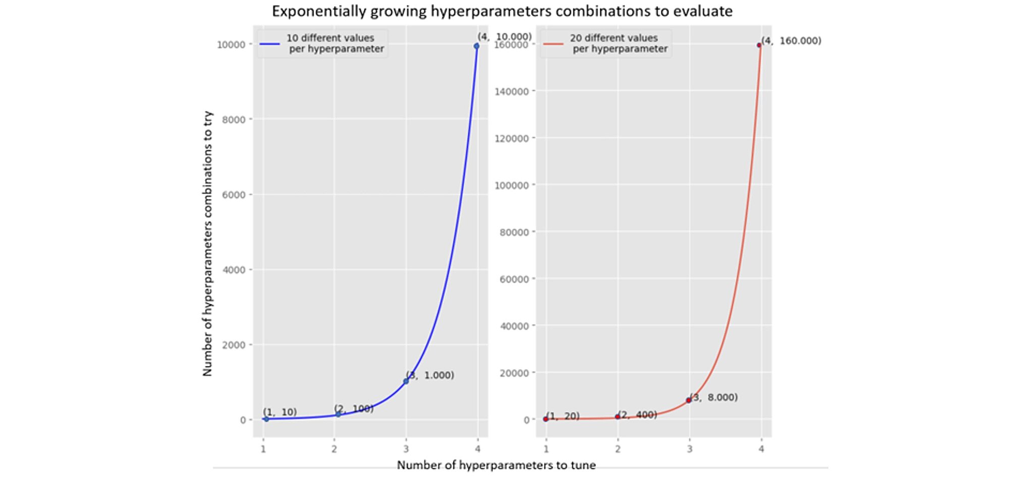
Why not try all possible values for all hyperparameters and see which combinations give the best score? This would guarantee we find the hyperparameter vector that gives our algorithm the best performance. However, in practice we do not have unlimited time and/or computing resources and the hyperparameter space is often not discrete but continuous.
The number of hyperparameter combinations grows exponentially with more hyperparameters (see two graphs below). The left-hand graph shows 4 hyperparameters and 10 different values which requires 10.000 tries (training the model and evaluating the objective function, we use the Poisson deviance). The required number of tries increases to 160.000 when 20 different values are tested.
Hence developing an optimisation method that can find an optimum quicker is an area of focus in the field of machine learning.
The random search is easily implementable and intuitive. However, it does not guarantee finding satisfactory local minimum quickly. Nor does it learn information from the previous iterations to target the search unlike the following two methods which leverage on the information collected during the previous iterations.
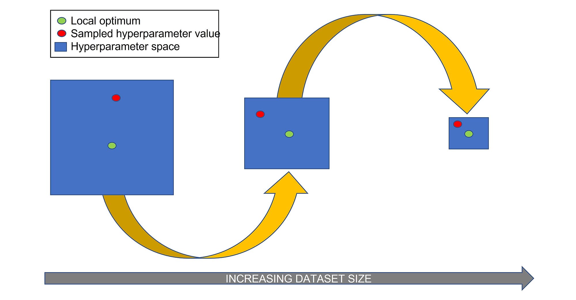
Halving random search is similar to random search, but it does not train the algorithm with randomly selected hyperparameters on the whole training set, but only on a small portion. In the next iteration it increased the portion of training data by randomly sampling from hyperparameter combinations that led to satisfactory results. The steps of the algorithm are as follows:
Bayesian Search works similarly to Halving Random Search as it keeps track of the information collected during the optimisation process. However, instead of trying to evaluate the objective function around the area which gave the lower scores randomly, it attempts “guessing”, mapping and modelling the probabilistic function between the scores and its hyperparameters. This is also often referred to as the surrogate model of the objective function. The surrogate model can be any probabilistic model fitting a Gaussian distribution.
Why use another proxy model on top of the existing model which effectively corresponds to an optimisation within an optimisation? Firstly, the surrogate model is easier to optimise than the objective function; it takes less time to evaluate because it maps a probability function between our loss scores and the hyperparameters values. Secondly, as we fit a Gaussian process, we have a measure of uncertainty of the distribution of the loss function with respect to its hyperparameter space.
The Bayesian hyperparameter optimisation algorithm works as follows:
This method may require less iterations to find the optimal set of hyperparameter values, because it does not search in the irrelevant/suboptimal areas of the hyperparameter space.
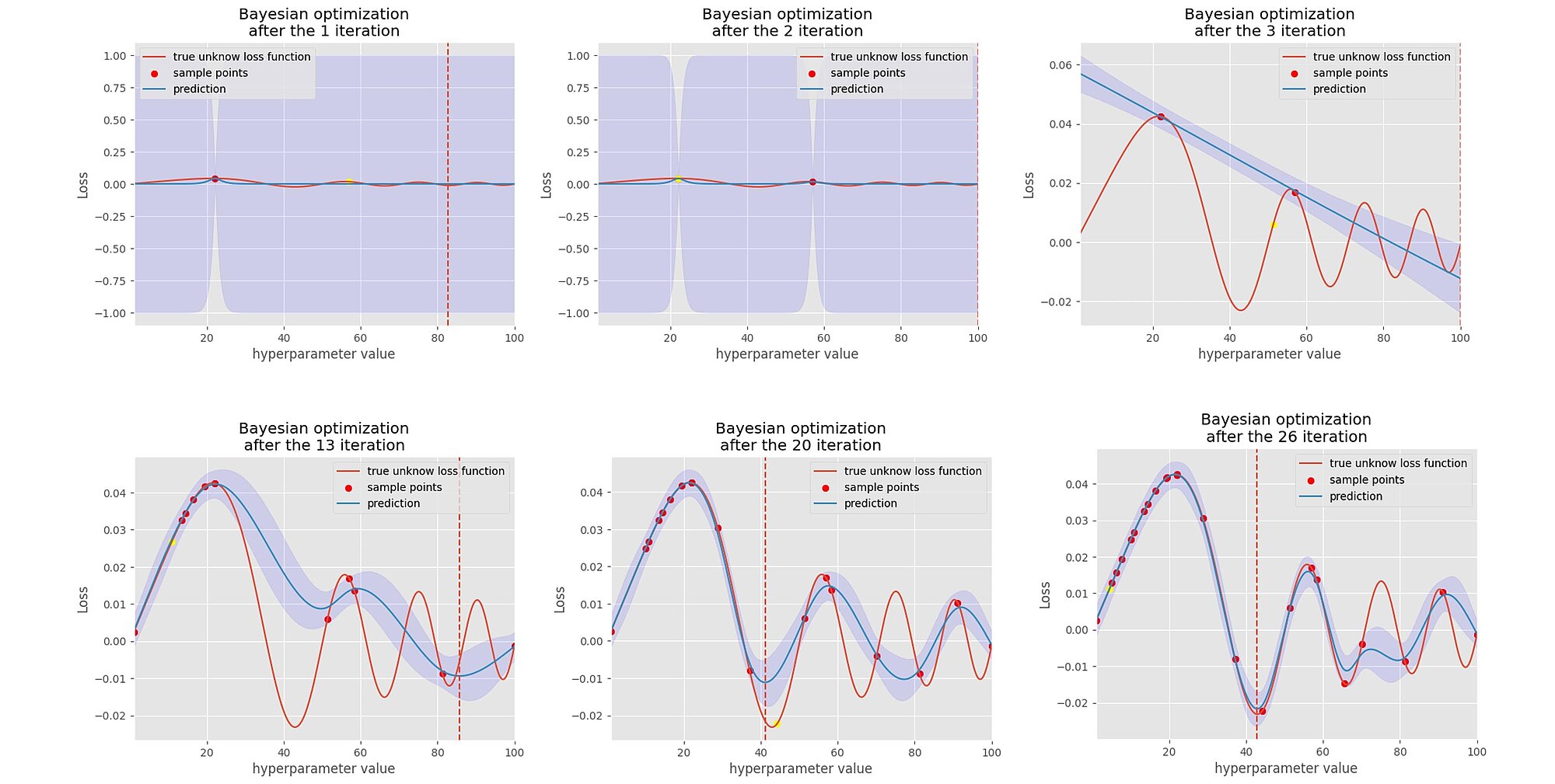
In the graphs below, we can see that we sample one point at a time, then we fit a Gaussian process on this point, then through an acquisition function we select the second next point to evaluate and sample the loss score. As we iterate through, the acquisition function helps to search in the area where it believes there are more chances of improvement and avoid areas where there is too much uncertainty about the loss function. Little by little, it finds the minimum of the loss function and its uncertainty decreases.
Although in theory the Bayesian optimisation technique seems more attractive, it is not empirically proven that it outperforms the random search as we will see later. All HOMs were model agnostic as we can apply those techniques to any estimators.
Having discussed the optimisation techniques, let us talk about the algorithm to optimise.
Regression trees are binary trees that recursively split the dataset down to the “leaf” nodes (final nodes) which corresponds to data with only one homogeneous class. The data is partitioned recursively based on one or more if-then statements for the features. It is used to forecast the value of a continuous variable (the number of claims of a policyholder for example).
Below is an example of a tree:

Here is an example of a non-optimized regression tree trained on the train dataset:

How this was this accomplished?
All the data is within the same space or region.
It is computationally infeasible to consider every partition of the feature space into j boxes. One possibility to overcome this limitation is to go for a top-down, greedy approach known as recursive binary splitting. The approach is top-down as it starts at the top of the tree (where all observations fall into a single region) and successively splits the predictor space into two new branches. This approach is also greedy as at each step the algorithm chooses the best split at that region regardless of the next steps (the steps in the branches further down).A selection of the predictor and the cut point that leads to the greatest reduction in loss function is needed to perform the recursive binary splitting.
However, the process described above can overfit the data and perform poorly on test set. The overfit model produces high variance. A smaller tree with fewer splits may lead to lower variance with better interpretation but higher bias.
One way to address this problem is to split the nodes if they result in a decrease in the loss function. This strategy works sometimes but not always. Tree size is a tuning hyperparameter governing the model’s complexity and the optimal tree size should be attuned to the data itself. To overcome the danger of overfitting the model, we apply the cost complexity pruning algorithm.
Pruning a branch of a tree T means collapsing all descendants nodes from a node t.
The idea is to develop the largest possible tree and then stop the splitting process when some minimum node size (usually five) is reached. The cost complexity measure of a tree T is the following:

Where:
D is the loss function or Deviance Poisson in the insurance case
τ is a set of indices for labelling terminal nodes
ĉt=mean(yi|xi ∈ χt), t ∈ τ with
yi the ith dependent variable
xi the ith explanatory variable
χt the subspace from node t
the number of terminal nodes |T| is called the complexity of the tree T
α is the increase in the penalty for having one more terminal node.
The tuning parameter governs the tradeoffs between tree size and its quality of fit. Large values of αresult in smaller trees (and vice versa). This process is analogous to the procedure in ridge regression, where an increase in the value of tuning parameters will decrease the weights of coefficients.
The advantages of a regression tree model are:
There are also some drawbacks:
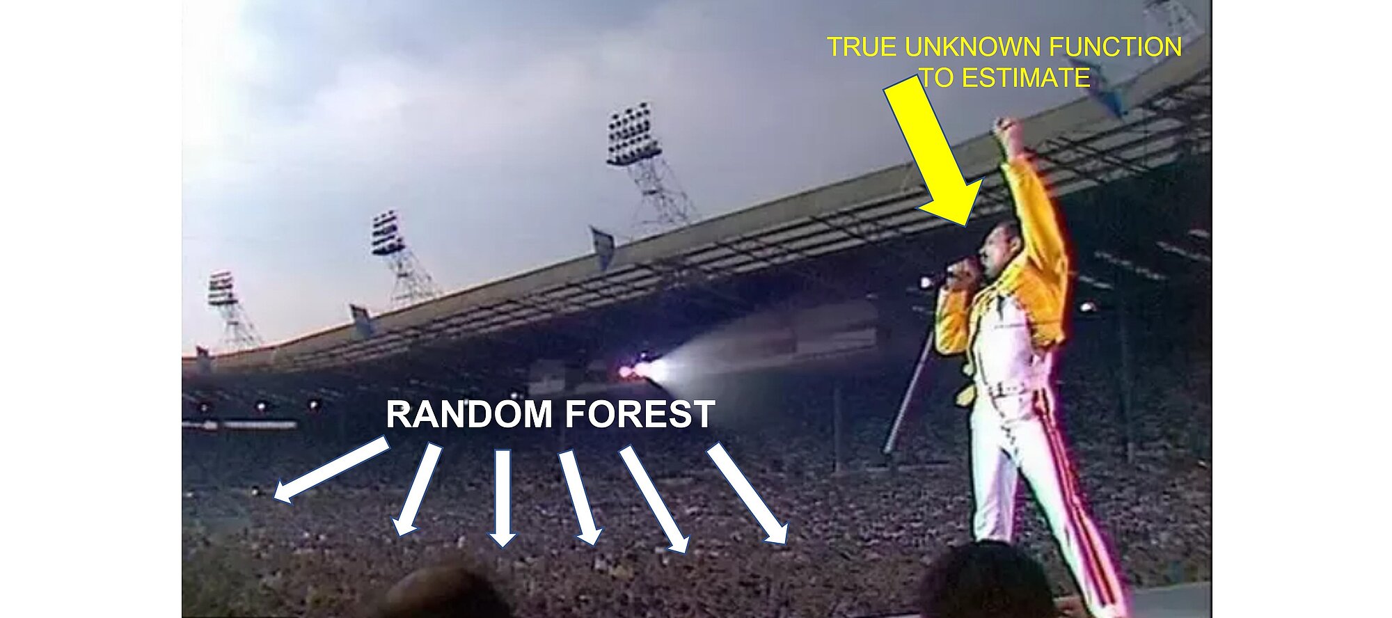
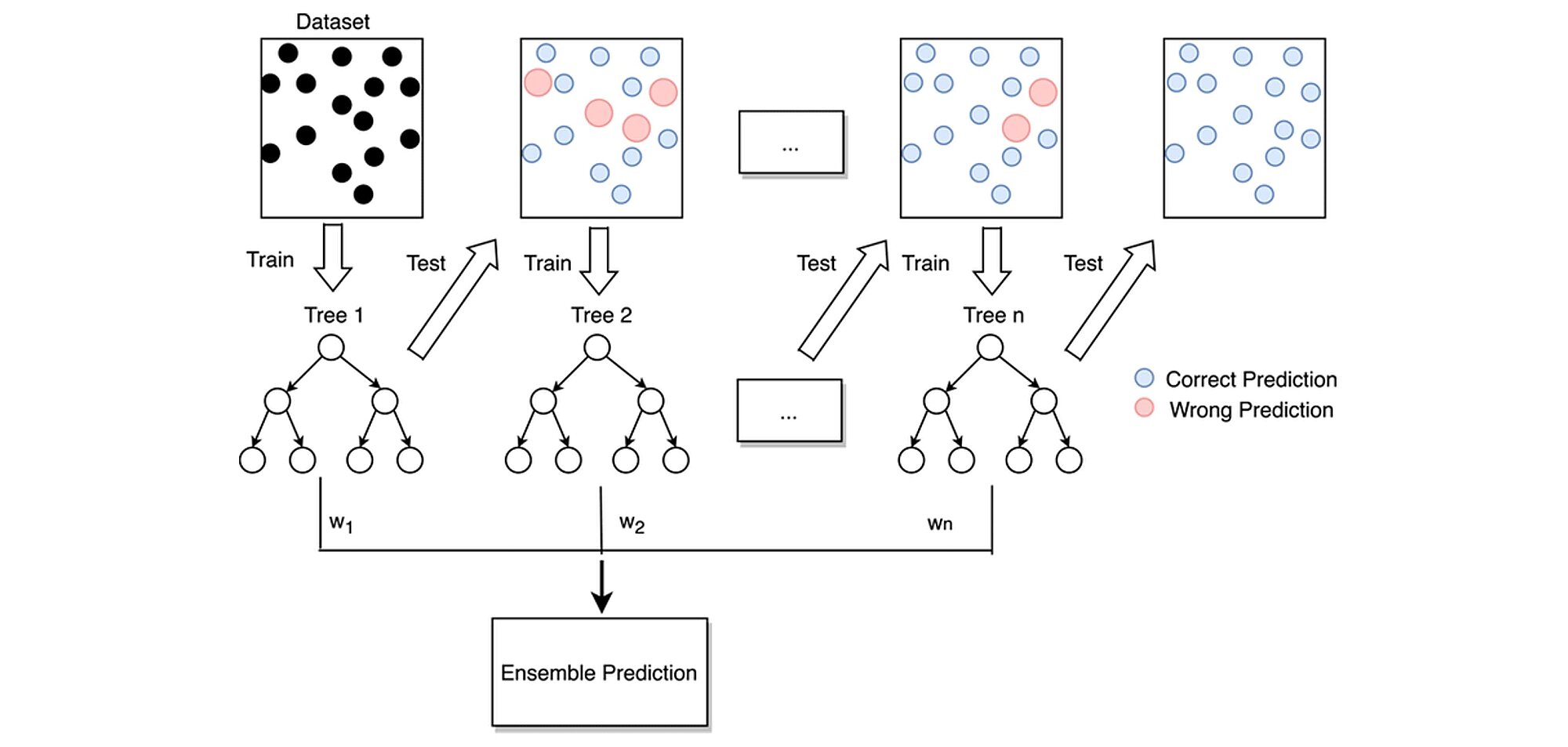
Random Forest is one of the ensemble learning methods which share a common intuition: what do you do if the doctor tells you that you have a serious illness that requires surgery? Despite the doctor's expertise, you may want to consult other specialists because his opinion alone may not be convincing enough. Ensemble methods work on the similar principle. Instead of having one single estimator that does everything, we build several estimators of lesser quality and aggregate their opinions and predictions into one to make the right decision. Each estimator has a fragmented view of the problem and does its best to solve it. These multiple estimators are then put together to provide a global view. The assembly of all these estimators that makes algorithms like random forest extremely powerful.
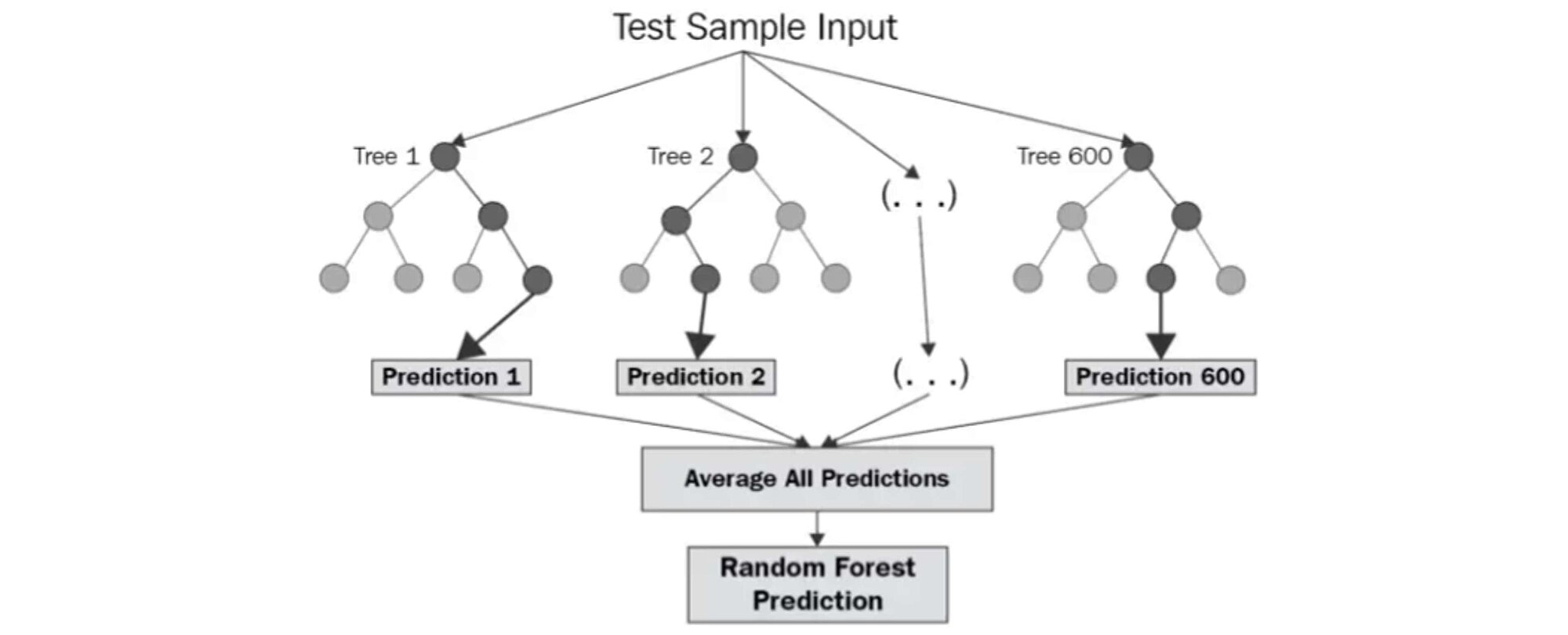
Source: levelup.gitconnected.com/random-forest-regression-209c0f354c84
The diagram above shows the structure of a Random Forest. You may notice that the trees run in parallel without interaction between them. A Random Forest operates by constructing several decision trees during training time and outputting the mean of the classes as the prediction of all the trees.
Decision trees have an architecture that allows them to fit perfectly to the training data. However, after a certain point, the model becomes too influenced by the training data, which can lead to biases. The use of several trees offers more flexibility and reduces this problem. This follows the wisdom of crowds principle, where a higher form of intelligence emerges from a group of people. For example, at a concert, the audience always sings in tune while most people sing out of tune. Each person corrects the mistakes of their neighbors.
The random forest (RF) algorithm creates a series of decision trees (a drill). Each tree considers a randomly selected part of the features. Several hyperparameters are to be defined and can be adjusted to ptimiza the algorithm. The most important are:
The steps for building a random forest are:
Because the trees can be constructed to run in parallel, the training and optimization time of a Random Forest algorithm can significantly speed up using jobs optimization as we will see in following sections.
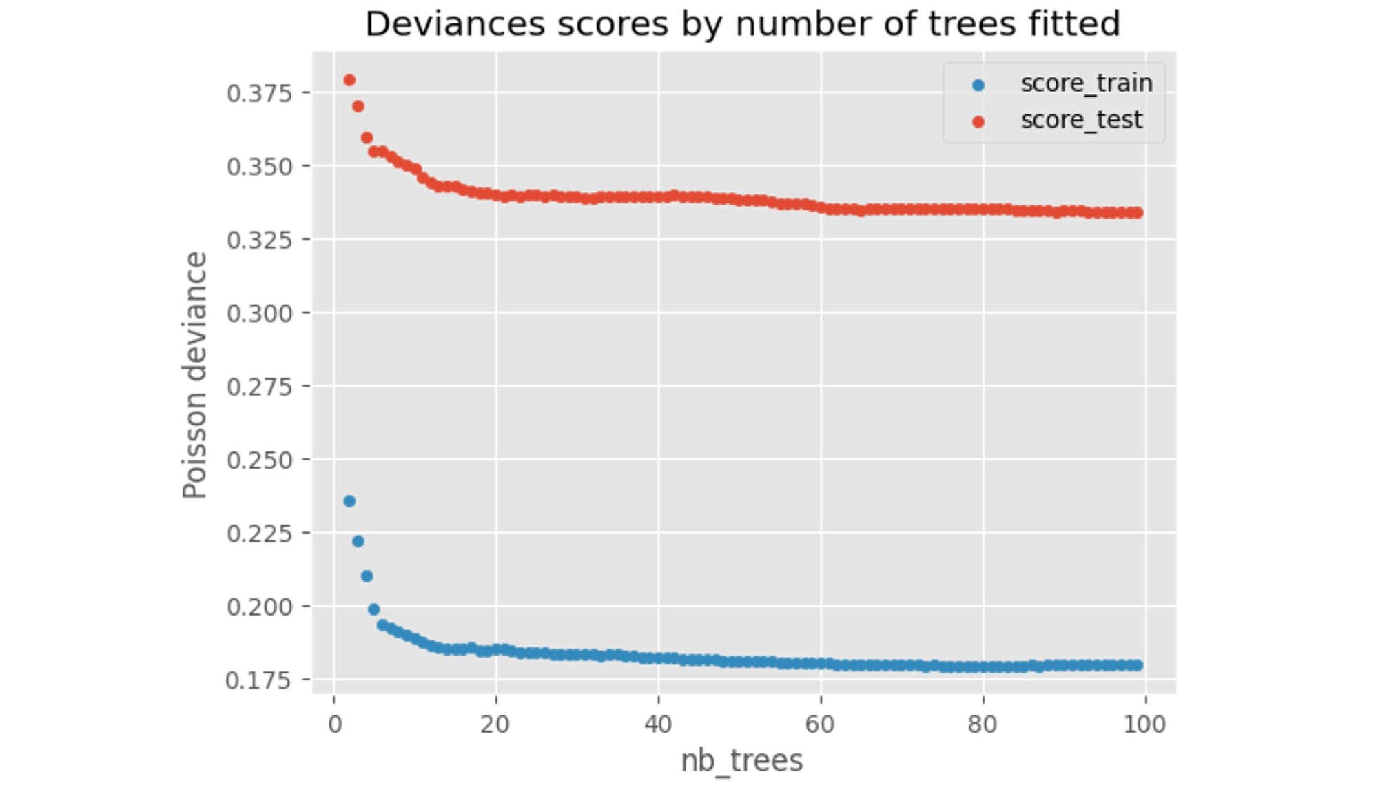
We can check how the performance on the training and test set behaves as we increase the number of trees fitted.
We can observe that above 80 trees, no further significant performance gains are achieved.
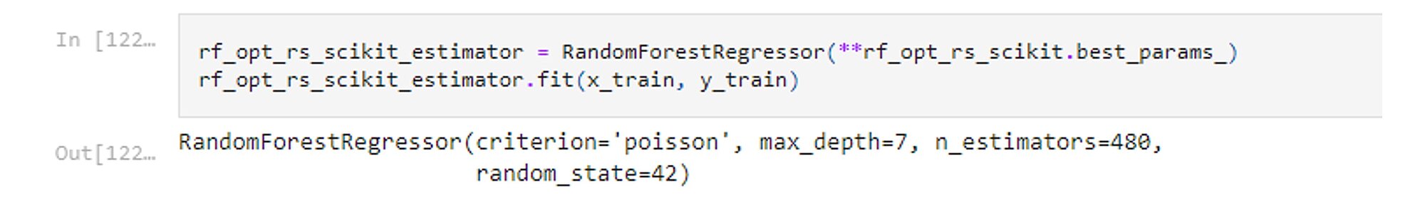
We must fine tune these different hyperparameters.
To give an example, after running the Random search hyperparameter optimization using Scikit-Learn, we can fit the optimal model with criterion = Poisson and max_depth=7 and number of trees= 480 as those values were deemed optimal by the HOM.
We can now interpret the model and we start by determining the importance of the variables. As seen in the regression trees, an importance index provides a ranking of the variables from the most important to the least important ones. If a variable is used by a significant number of trees and is higher-up in the trees, then it is deemed more important.
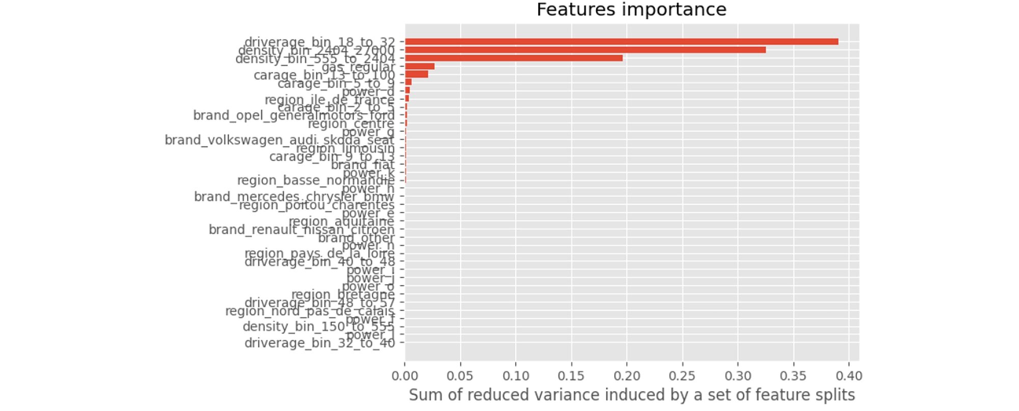
This last graph tells us that the 2 variables that contribute the most to our model are driverage_bin_18_to_32 and density_bin_2404_2700. Similarly, when we are younger, we are less experienced drivers and are more likely to have an accident. Also, the more crowded is the area, the heavier the traffic and the higher the odds of an accident.
Like random forest, gradient boosting belongs to the family of the ensemble methods. Any estimator can be boosted, but here we will focus on boosting a regression trees. While random forest builds several trees in parallel, boosting also builds k trees (or other basic algorithms), but it does so serially. The tree k + 1 has access to the errors of its predecessors. Therefore, it is aware of the past errors and focuses on correcting them. For a classification problem, the prediction is not a majority vote, but a weighted sum of the weak algorithms (the final decision is based on the weighted average of the individual predictions).
This model is based on a sequential approach called adaptive which consists in combining several models with weak predictive powers (weak learners) to obtain a model with a powerful predictive power.
The graph below summarises how this model works:
Parameterisation of gradient boosting algorithms is not easy. Compared to random forest, it has the disadvantage of being iterative and therefore unsuited for parallelisation. In other words, the search for the right parameters can be long.
Let us go through the most important parameters (many are common to the RF algorithm):
loss: the cost function that we aim to minimise; an important criterion, but in our case, this parameter is fixed.
n_estimators: the number of estimators or iterations you will do. To set it, observe the train and test errors: if you do not overfit, increase the number of estimators. It is common to have hundreds of estimators.
max_depth: The depth of the trained trees. Trees are shallow compared to the random forest, from three to eight in practice. You can already get reliable results with trees with depth of two (also called stump trees), with only one split!
Another important boosting-specific hyperparameter is:
learning_rate: Step size shrinkage used in update to prevent overfitting. After each boosting step, we can directly get the weights of new features, and the learning rate (also called eta or shrinkage parameter) shrinks the feature weights to make the boosting process more conservative.
In our example we define a grid which contains the maximum depths of trees and the number of estimators.

Each model is built with different number of trees. We then compare them using a validation sample estimation or cross validation. Based on that, we can select our best model.
The loss function can be approximated by being sampled after evaluating the models for a few hyperparameters values. By varying the n_estimators and learning_rate hyperparameters, we can guesstimate where a local minimum stands. In the example below n_estimators is in [20,30] and learning_rate [0.2, 0.3]
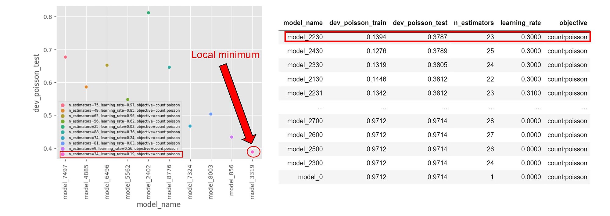
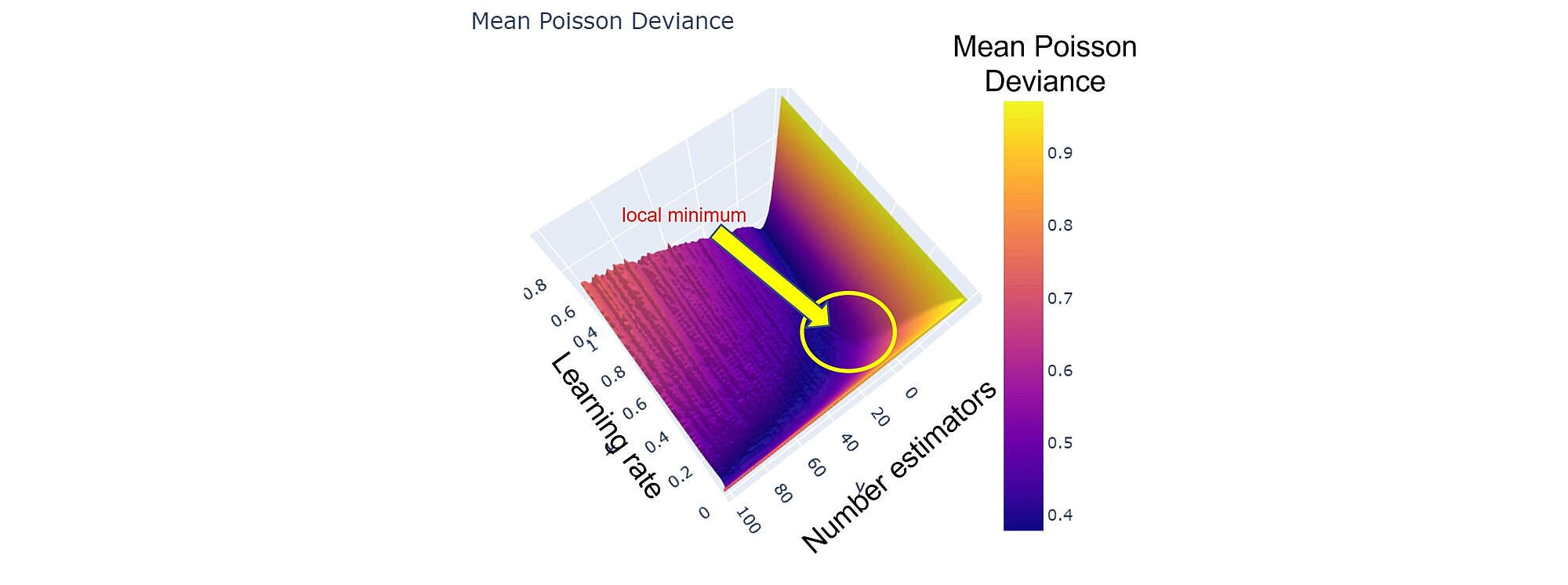
Note that the results are run on a larger training dataset and might differ from those displayed here. However, getting a grasp on where our local minima might be on smaller samples can be useful for initialising our optimisation searches.
Neural networks (NNs) are useful for modeling multiple variables interactions and complex non-linear relationships. While logistic regression can handle variables interaction if specified and tree-based methods can discover it through subsequent splits, it is practically impossible to find and guess all the interactions and relationships between variables and the expected outcome. We need a model that can approximate any complex function without requiring the model user to "guess and specify" all the interactions between the variables relative to the expected number of claims. This is what neural networks do.
Thanks to the universal approximation theorem (see Kurt Hornik and HalbertWhite, 1989 and Cybenko, 1989) we do not need to design a specialised model family for each problem. Neural networks offer a universal approximation framework. The theorem states that a neural network with a linear output layer and at least one hidden layer on which any "squashing" activation function is applied can approximate any continuous function (Borel measurable) from one finite-dimensional space to another with a desired error tolerance.

However, how can a neural network approximate any continuous function? The neural network can cut the input space into numerous (non-)linear regions. The number of linear regions grows exponentially with the number of layers. For a NN of 5 layers and 5 neurons per layer, the NN can discriminate between 38,146 separate groups:
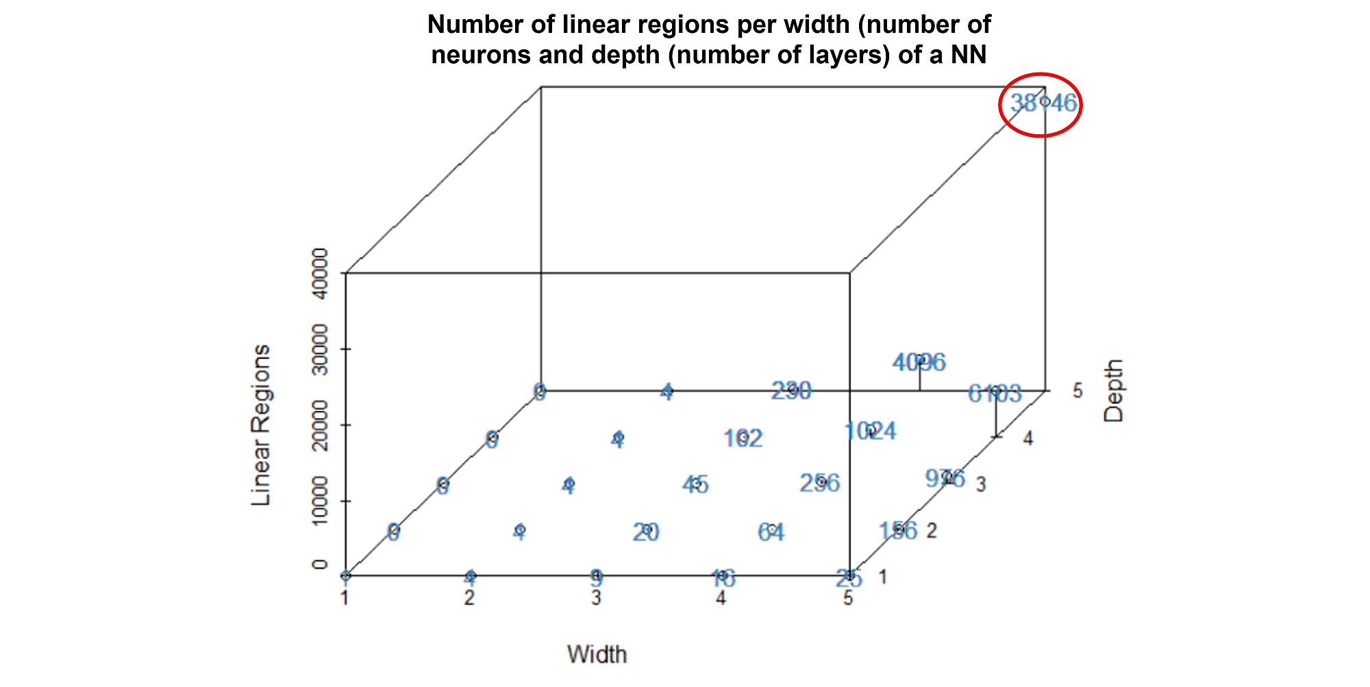
The more layers you add to your neural network, the greater its capacity but also the greater the risk of overfitting. That is why hyperparameter tuning is crucial when training a NN.
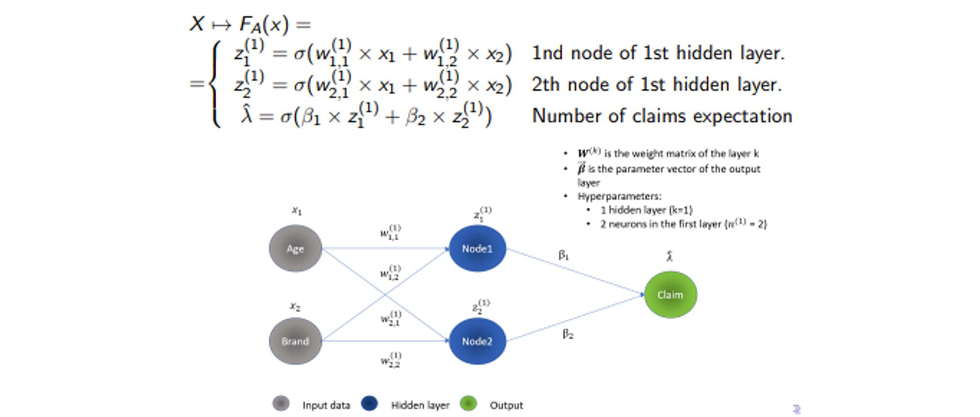
Let us look at how NNs work from a mathematical standpoint. NNs are essentially nested, intricated linear algebraic operations. Each layer of the neural network is a non-linear transformation of a combination of previous nodes interactions that are themselves also nonlinear transformations of previous nodes and the input space.
A graphical illustration of inference for a feed-forward neural network:
The NNs possess a greater model capacity. However, this comes at the cost of interpretability even though there has been a substantial progress as regards Deep Learning interpretability. This will be covered in our upcoming blog post which will show how under specific conditions, NNs are equivalent to decision trees. Despite the recent advancements in AI interpretability, NNs are still considered as “black-box models.”
Another issue with NNs is the number of parameters and hyperparameters to train. In the example below, with only two input variables, one layer of two neurons, there are 6 parameters to train. However, the number of hyperparameters to train in a NN is even greater: number of layers, neurons per layer, activation functions, optimizer, learning rate, epochs, batch size, etc.
In the table below, you will find an aggregation of the results for the different model classes along with the performance metrics realised on the train and test dataset, the optimisation time and the best hyperparameters selected.
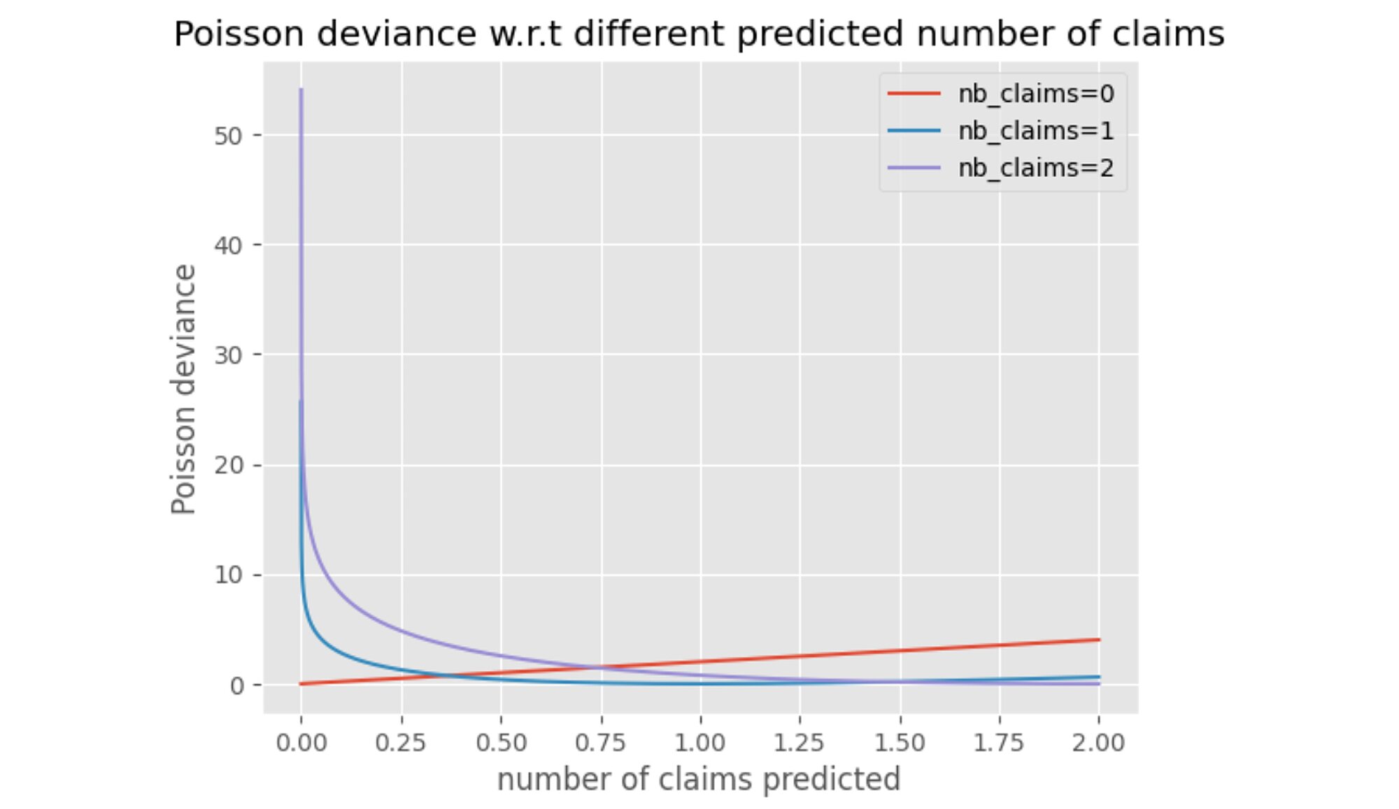
The deviance poisson was evaluated on both train and test sets. The lower the deviance the better the fit. The mean poisson deviance formula used offset by the contract exposure is:

Where:
Note the Poisson deviance penalizes more when the prediction is below the true observed number of claims and less above.
When possible, the standard deviation of the cross-validation deviance losses gathered during the hyperparameter tuning was collected. It indicates how stable the estimator is. The optimization time is in minutes and the optimization was performed on an Intel Core i5 CPU.
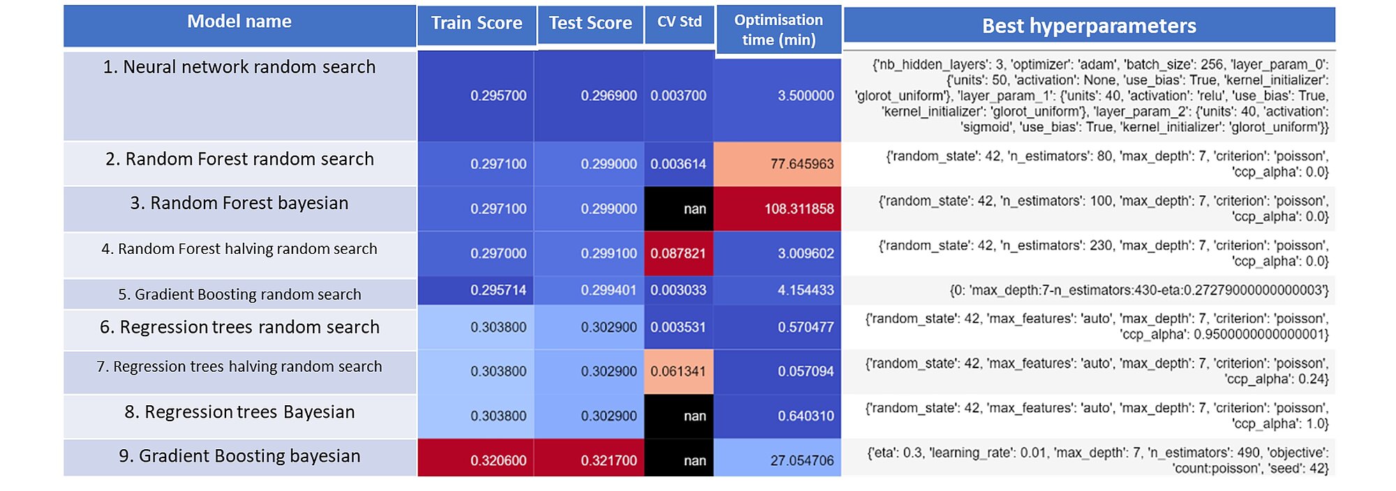
The neural network optimised with a random search procedure performed the best. Second and third positions are occupied by two random forest models optimised with random search and Bayesian searches respectively. As a benchmark, we optimised a logistic regression model and reached 0.3108 poisson deviance score on the test set.
Our test shows that the machine learning algorithm outperforms traditional logistic regressions (that we described in the previous article). This comes at the cost of computation time and interpretability. However, we can see that the computation time can be satisfactorily reduced using the appropriate hardware and parallelization. This can be further improved through the wise choice of hyperparameters – interestingly the optimization method used for that purpose had no significant impact; the more sophisticated hyperparameter optimization techniques did not perform significantly better than the simple ones. As regards the model, we can note that the NN model outperformed all others. However, NN have the greatest problem with interpretability. In the next blogpost we will tackle the problem of interpretability and how to address it.
Finalyse InsuranceFinalyse offers specialized consulting for insurance and pension sectors, focusing on risk management, actuarial modeling, and regulatory compliance. Their services include Solvency II support, IFRS 17 implementation, and climate risk assessments, ensuring robust frameworks and regulatory alignment for institutions. |

Check out Finalyse Insurance services list that could help your business.
Get to know the people behind our services, feel free to ask them any questions.
Read Finalyse client cases regarding our insurance service offer.
Read Finalyse blog articles regarding our insurance service offer.
Designed to meet regulatory and strategic requirements of the Actuarial and Risk department
Designed to meet regulatory and strategic requirements of the Actuarial and Risk department.
Designed to provide cost-efficient and independent assurance to insurance and reinsurance undertakings
Finalyse BankingFinalyse leverages 35+ years of banking expertise to guide you through regulatory challenges with tailored risk solutions. |

Designed to help your Risk Management (Validation/AI Team) department in complying with EU AI Act regulatory requirements
A tool for banks to validate the implementation of RWA calculations and be better prepared for CRR3 in 2025
In 2027, FRTB will become the European norm for Pillar I market risk. Enhanced reporting requirements will also kick in at the start of the year. Are you on track?
Finalyse ValuationValuing complex products is both costly and demanding, requiring quality data, advanced models, and expert support. Finalyse Valuation Services are tailored to client needs, ensuring transparency and ongoing collaboration. Our experts analyse and reconcile counterparty prices to explain and document any differences. |

Helping clients to reconcile price disputes
Save time reviewing the reports instead of producing them yourself
Helping institutions to cope with reporting-related requirements
Be confident about your derivative values with holistic market data at hand
Finalyse PublicationsDiscover Finalyse writings, written for you by our experienced consultants, read whitepapers, our RegBrief and blog articles to stay ahead of the trends in the Banking, Insurance and Managed Services world |

Finalyse’s take on risk-mitigation techniques and the regulatory requirements that they address
A regularly updated catalogue of key financial policy changes, focusing on risk management, reporting, governance, accounting, and trading
Read Finalyse whitepapers and research materials on trending subjects
About FinalyseOur aim is to support our clients incorporating changes and innovations in valuation, risk and compliance. We share the ambition to contribute to a sustainable and resilient financial system. Facing these extraordinary challenges is what drives us every day. |

Finalyse CareersUnlock your potential with Finalyse: as risk management pioneers with over 35 years of experience, we provide advisory services and empower clients in making informed decisions. Our mission is to support them in adapting to changes and innovations, contributing to a sustainable and resilient financial system. |

Get to know our diverse and multicultural teams, committed to bring new ideas
We combine growing fintech expertise, ownership, and a passion for tailored solutions to make a real impact
Discover our three business lines and the expert teams delivering smart, reliable support