Statistical techniques have been used in building credit models. Below are some of the most common techniques like regression, linear programming, logistic regression, k-nearest neighbor, random forest trees etc.
Linear regression is a method describing the relationship between a response variable and independent variables by a linear relationship. It assumes a straight-line relationship between dependent and independent variable. It is used to predict the continuous variables like age, income, amount etc. It is estimated by a technique called ordinary least square (OLS), which is about identifying the line that minimize the sum of square differences between points on the estimated line and actual values of independent variable.
Logistic regression has long been one of the most widely used statistical techniques. The method differs from linear regression in the sense that the dependent variable in logistic regression is of dichotomous (0/1) form. Logistic equation is estimated by a technique known as maximum likelihood estimation (MLS), such that joint probabilities of observing the actual event is maximized or sum of log likelihood is maximized.
Clustering is when segmentation on the dataset is done such that homogenous clusters are made i.e. objects within a group are similar to each other and different from the object in another group and next credit scoring can be done on each homogeneous segment.
K-Nearest Neighbor (KNN) determines in which group data-points will fall into by determining how close a data- point is to a group, that is it will fall into that group which is closest to it.
Random Forest is a combination of tree predictors where the values of a random vector of each tree are sampled independently and have the same distribution for all the trees in the forest.
Below are some of the criteria in evaluating performance.
Confusion matrix - It looks at how often the model has correctly predicted an event. The average correct classification rate measures the percentage of good and bad credit ratings in a dataset.
There is an estimated misclassification cost in which lenders reject loans applications which is actually good (so- called false negatives) or accept a loan application which is actually bad (so-called false positives) lead to misclassification. As a result, it leads to Type 13 and Type 2 error4. Sensitivity is also called as recall which is true positive divided by true positive plus false negative whereas specificity (also called as precision) is the ratio of true positive to true positive plus false positive.
| Predicted Class | |||
|---|---|---|---|
Actual Class | Class 0 | Class 1 | |
| Class 0 | True negative | False positive | |
| Class 1 | False negative | True positive | |
Class 0= Non-default, Class1=Default
True negative - When obligor has not predicted default and in actual not defaulted also.
False negative - When obligor has predicted not default but in actual has defaulted.
False positive - When obligor has predicted defaulted but in actual has not defaulted.
True positive - When obligor has predicted default and in actual has defaulted also.
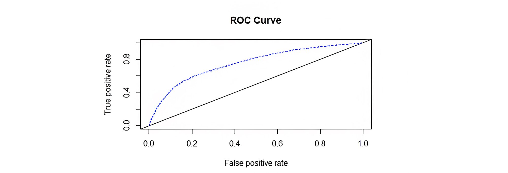
Receiver Operating Characteristic (ROC) - has long been used to detect true and false rates of classification. It is a graph of sensitivity (true positive) on y-axis and specificity (false positive) on the x-axis. Sensitivity represents bad customer classified as bad and specificity represent good customer classified as bad.
The closer the curve to the y-axis (the true positive) the better the model is. The so-called Area under the curve (AUC) in the ROC plot serves as a better performer than overall accuracy as the latter is based on a specific cut-off point while ROC takes all the cut-off point and thus plot sensitivity and specificity plot.
Thus, in short, when we compare the overall accuracy, we are measuring the accuracy based on some cut-offs point which concludes that accuracy varies for a different cut-off point. By default, the cut-off point is 50%.
Below is the diagram of ROC curve. In conclusion, the higher the AUC (area under the curve), the better the model is.
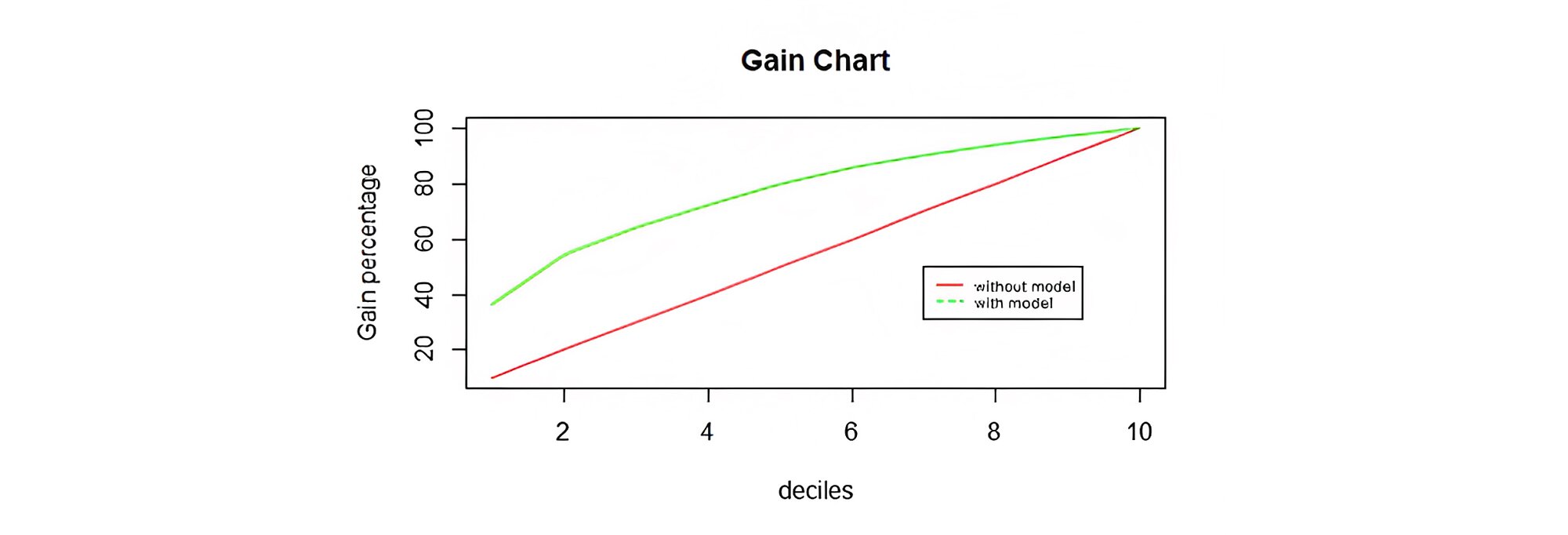
Gain chart - It is used to determine how much better one can do with predictive models than without. In this, validation sample is scored (predictive probability) and then ranked in descending order by predictive probability. The ranked file is then split into deciles such that an equal number of observations are there in each decile and then the cumulative number of actual events are taken with a conclusion that the predictive outcome should come higher than the observed outcome for better model accuracy.
In other words, the higher the percentage of observations in the first few deciles, the better the predictive power of the model.
P-value is important metric to determine statistical significance of any variable, All the independent variables with P value of less than 5% (rejecting the null hypothesis) are statistically significant and are included in the model. In other words, the independent variables have an influence on the dependent variable and the rest of the variables which are not included in the model are having P-value greater than 5% and are deemed insignificant and does not have influence on the dependent variable.
R-square explains what proportion of variance in dependent variable is being explained by independent variable. Higher the R-square, the better the model is. The disadvantage of using R-square is as more independent variables get added, R square will go up irrespective whether the variable is significant or not. So, adjusted R-square is being used as it will go up only if significant variable is added to the model.
There are some regression assumptions
If all the above conditions are met, then it is called as BLUE (Best linear unbiased estimator) model.
Homoscedasticity - It is when residuals should have constant variance i.e., it should not show any pattern, if the model is not homoscedastic then it will get biased and will affect the performance of the model.
Multicollinearity - There should not be any correlation between independent variables because if 2 independent variables are highly correlated with each other, then they both are having the influence on the dependent variable and that may affect the performance of the model. It’s VIF (Variance inflation factor) which is being used as a measure gauge multicollinearity and should be less than 3 for better models.
Stationarity testing - It is a test to check that the mean and variance of the time series should be constant over tine.
Using R tool, using 4 algorithms - Logistic regression, Random Forest, clustering and KNN, models got developed and compared with each other using the above performance evaluation metrics based on a sample banking dataset containing bureau and demographic fields.
Data
Data taken is a sample of anonymous banking data with 150000 datapoints with 11 variables. Demographic variables are like ‘Age’ and ‘Number of dependents’ whereas credit bureau variables like – ‘Revolving utilization of unsecured loan’, ‘Number of 30.59 days past due not worse’, ‘Debt ratio’, ‘Monthly income’, ‘Number of open credit lines or loans’, and ‘Number real estate loans or lines.
For building models, it is important to have training and testing (validation) dataset. If there is one single dataset, by a thumb rule, it should be divided to at least 70:30 ratio. 70% in training and 30% in testing dataset. The result of the model is applied on the testing dataset to check upon how well the accuracy of the model or in other words how well the model is performing on unseen data.
Logistic model
Two iterations of the Logistic Regression model were done as in the first iteration some of the variables were statistically insignificant, thus retaining only those variables which were statistically significant (i.e. those variables with P - Values less than 5% namely - ‘number of 30_59dayspastduenot worse’, ‘number of open credit lines and loans’, ‘number of dependents’, ‘monthly income’ and ‘age’) and doing the iteration second time to check for statistically insignificant variable if any. There is no statistically insignificant variable was found in the second iteration with the help ‘glm’ function in R as shown below.
| Coefficients: | ||||
|---|---|---|---|---|
| Estimate Std. | Error | z value | Pr (<|z|) | |
| (Intercept) | -1.802991 | 0.084297 | -21.389 | < 2e-16 *** |
NumberOf Time30.59Days PastDueNotWorse |
1.014009 |
0.015124 |
67.047 |
< 2e-16 *** |
NumberOfOpen CreditLines AndLoans |
-0.026735 |
0.002843 |
-9.405 |
< 2e-16 *** |
| Number Of Dependents | 0.060666 | 0.011063 | 5.484 | 4.16e-08 *** |
| monthly Income | 0.368350 | 0.075812 | 4.859 | 1.18e-06 *** |
| age | -0.028723 | 0.001022 | -28.102 | < 2e-16 *** |
The accuracy in the test dataset and area under the ROC curve as shown in Figure 1 are found to be 72.8% and 75.4%. respectively, whereas the accuracy in the training dataset is 74%. The Gain Chart showings that the first decile has 36.5% of good customers and reaching above 50% in the second decile that is 54.4%. Thus, concluding that the higher the percentage of observations in the first few deciles, the better the predictive power of the model is as mentioned earlier as well in the above section.
The confusion matrix shows 30036 as True Negative (TN), 1871 as True Positive (TP), 10867 as False Negative (FN) and 1049 as False Positive (FP) as shown in Table 3 below.
| Predicted Class | |||
|---|---|---|---|
| Actual Class | Class 0 | Class 1 | |
| Class 0 | 30036 (TN) | 1049 (FP) | |
| Class 1 | 10867 (FN) | 1871 (TP) | |
Here, the recall is 14.6%.
The AUC with only demographic and credit bureau variables considered separately and examined, come out to be 63.69% and 71.6% respectively, indicating credit bureau variables explaining dependent variable more than demographic variables.
The top 5 factors influencing the dependent variable are- ‘Number Of 30.59 Days Past Due Not Worse’, ‘Monthly Income’, ‘Number of Dependents’, ‘age’ and ‘Number of open credit lines or loans.
The incorporation of variables changes the performance of the model
| Variables | AUC (Area under the curve) |
|---|---|
| Number of 30.59 days past due not worse | 68.3 % |
| Number of 30.59 past due not worse+ number of open credit lines or loans | 71.1 % |
| Number of 30.59 past due not worse+ number of open credit lines or loans+ number of dependents | 71.1 % |
| Number of 30.59 past due not worse+ number of open credit lines or loans+ number of dependents+ monthly income | 71.8 % |
| Number of 30.59 past due not worse+ number of open credit lines or loans+ number of dependents+ monthly income +age | 75.4 % |
Random Forest
The area under the curve of ROC curve was found to be 80% as shown in Figure below with 93.3% accuracy in the test dataset and 95% accuracy in the training dataset.

The confusion matrix in Table below shows that 183 are True Positives (TP), 40726 are True Negatives (TN), 166 as False Negatives (FN), and 2748 as False positives (FP) –
| Predicted Class | |||
| Actual Class | Class 0 | Class 1 | |
| Class 0 | 40726 (TN) | 2748 (FP) | |
| Class 1 | 166 (FN) | 183 (TP) | |
Here, the recall is 52.4% which is far better than logistic regression.
The top 5 Important variables in random forest which influence the dependent variable are ranked in descending order namely- ‘Revolutionising utilisation of unsecured lines or loans’, ‘debt ratio’, ‘age’, ‘number of 30_59 days past due. The below figure is giving the importance of variables based on mean decrease gini. Higher the value of mean decrease gini, more important the variable is in the model.
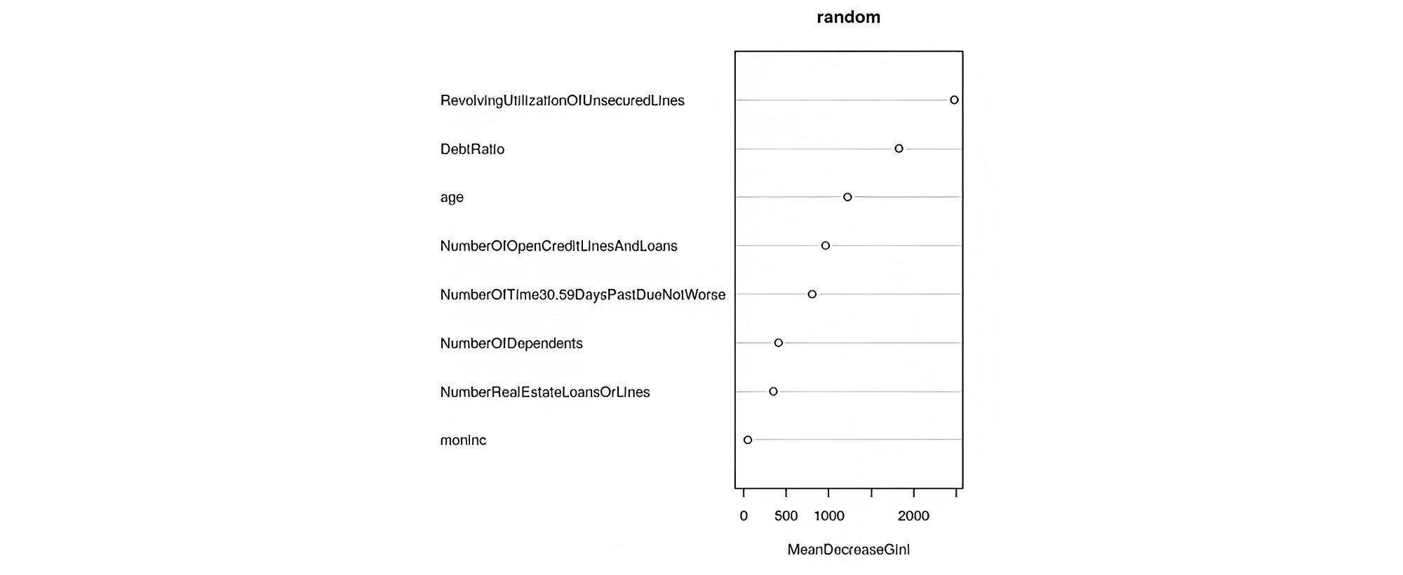
Variables like ‘revolutionising utilisation of unsecured lines or loans’ and ‘debt ratio’ were found to be the most important variables by the random forest method even though they are not statistically significant in logistic regression due to the latter’s limited ability to handle non-linear relationships (it is, after all a form of generalised linear model). So, a tree- based approach is a better one for handling variables with a non-linear relationship with the dependent variable.
K- nearest neighbor
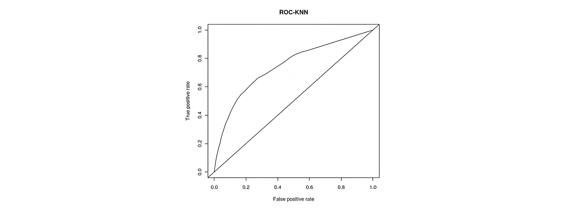
The AUC of ROC curve was found to be 74% as shown in figure below with accuracy of 93.13%, with K=23.
Confusion Matrix is shown in Table 6 below
| Predicted Class | |||
| Actual Class | Class 0 | Class 1 | |
| Class 0 | 40862 (TN) | 2849 (FP) | |
| Class 1 | 71 (FN) | 41 (TP) | |
Here recall is 36.6% which is better than logistic regression.
Clustering
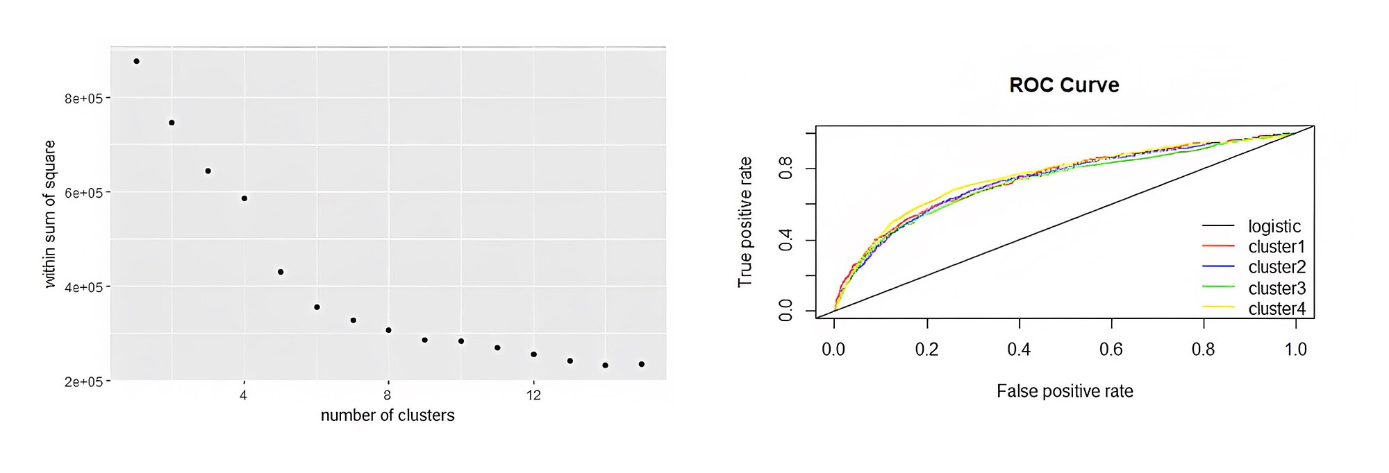
With the help of the K-means technique, clustering is done with the help of those variables which are statistically significant on normalized data. Clustering is done keeping in mind that the within cluster sum of squares should be as small as possible and between cluster sum of squares is maxima.
Hence, four clusters are made as up to 4 clusters as there is a good amount of fall in the within cluster sum of square as shown in Figure below, after which a logistic regression technique is applied on each cluster to check upon whether the performance of the model can be increased.
The AUC of cluster1, cluster2, cluster3 and cluster4 are coming out to be- 74.6%, 73.80%, 72.60% and 75.80% as shown in figure below Thus, it shows that the performance is not increasing beyond 75% with clustering.
We have seen that the performance of the model has increased in the case of random forest over logistic regression, logistic regression after clustering and KNN. The accuracy for random forest, logistic regression and KNN in the test dataset are 93.3%, 72.8% and 93.13% respectively. AUC for random forest is 80% while that of logistic regression and KNN are around 75%, thus showing an increase of 5% improvement in performance of random forest over logistic regression and KNN as shown in Figure below.

This may be due to as logistic regression is analogous to linear regression is analogous to linear relationship, so it’s not a perfect technique to have a good result for independent variables having non-relationship with dependent variable. So, for this, the tree-based approach is a better approach, here random forest is used which works better in handling influence of non-relationship of independent variable on dependent variables.
The area under the curve (AUC) is taken into consideration over the accuracy in determining the performance of the model as AUC takes all the cut-off point into consideration while the accuracy is based on a specific cut-off point, so the accuracy varies with different cut-off points. Performance did not increase beyond 75% even with a combination of clustering and logistic regression. On comparing random forest, logistic regression and KNN based on the recall, it tells that the recall of random forest is higher than the recall of other two techniques and the recall of KNN is higher than the recall of logistic regression.
Finally, it concludes random forest is best applied technique followed by KNN and logistic regression. Results could have been better with more data.
Finalyse InsuranceFinalyse offers specialized consulting for insurance and pension sectors, focusing on risk management, actuarial modeling, and regulatory compliance. Their services include Solvency II support, IFRS 17 implementation, and climate risk assessments, ensuring robust frameworks and regulatory alignment for institutions. |

Check out Finalyse Insurance services list that could help your business.
Get to know the people behind our services, feel free to ask them any questions.
Read Finalyse client cases regarding our insurance service offer.
Read Finalyse blog articles regarding our insurance service offer.
Designed to meet regulatory and strategic requirements of the Actuarial and Risk department
Designed to meet regulatory and strategic requirements of the Actuarial and Risk department.
Designed to provide cost-efficient and independent assurance to insurance and reinsurance undertakings
Finalyse BankingFinalyse leverages 35+ years of banking expertise to guide you through regulatory challenges with tailored risk solutions. |

Designed to help your Risk Management (Validation/AI Team) department in complying with EU AI Act regulatory requirements
A tool for banks to validate the implementation of RWA calculations and be better prepared for CRR3 in 2025
In 2027, FRTB will become the European norm for Pillar I market risk. Enhanced reporting requirements will also kick in at the start of the year. Are you on track?
Finalyse ValuationValuing complex products is both costly and demanding, requiring quality data, advanced models, and expert support. Finalyse Valuation Services are tailored to client needs, ensuring transparency and ongoing collaboration. Our experts analyse and reconcile counterparty prices to explain and document any differences. |

Helping clients to reconcile price disputes
Save time reviewing the reports instead of producing them yourself
Helping institutions to cope with reporting-related requirements
Be confident about your derivative values with holistic market data at hand
Finalyse PublicationsDiscover Finalyse writings, written for you by our experienced consultants, read whitepapers, our RegBrief and blog articles to stay ahead of the trends in the Banking, Insurance and Managed Services world |

Finalyse’s take on risk-mitigation techniques and the regulatory requirements that they address
A regularly updated catalogue of key financial policy changes, focusing on risk management, reporting, governance, accounting, and trading
Read Finalyse whitepapers and research materials on trending subjects
About FinalyseOur aim is to support our clients incorporating changes and innovations in valuation, risk and compliance. We share the ambition to contribute to a sustainable and resilient financial system. Facing these extraordinary challenges is what drives us every day. |

Finalyse CareersUnlock your potential with Finalyse: as risk management pioneers with over 35 years of experience, we provide advisory services and empower clients in making informed decisions. Our mission is to support them in adapting to changes and innovations, contributing to a sustainable and resilient financial system. |

Get to know our diverse and multicultural teams, committed to bring new ideas
We combine growing fintech expertise, ownership, and a passion for tailored solutions to make a real impact
Discover our three business lines and the expert teams delivering smart, reliable support