Machine Learning Model explainability – why it is important and methods to achieve it

Machine learning is today’s buzzword and it has gone through some phenomenal changes over the last few years. Starting as academic and research-oriented domain, we have seen widespread industry adoption across diverse domains including E-commerce, retail, Banking, Insurance, healthcare etc. Despite widespread adoption, machine learning models remain mostly black boxes. Hence  it is essential to have techniques for explaining these black boxes in an interpretable manner.

Should we just trust the machine learning model?
Or should we seek for the explanation of why it made a certain decision?
 

In “Little Britain”, a British sketch comedy show, a bank worker responds to customer requests by typing them into the computer and subsequently responding with "computer says no" without providing any explanations of the decision. In the world of more and more advanced AI systems it becomes clear that such attitude will not endure, as regulators demand more transparency to avoid possible biases based on factors as gender or race.

The concept of explainability is usually used in contrast to the “black box” term, that is a system e.g. algorithm where the user is only aware about the input and the output but has no insight into what is happening within the algorithm.

When it comes to methods such as machine learning, neural networks or AI the given systems can lack transparency or, what is worse, they can contain unconscious biases  of their creators. The issue is present also in ‘classical’ models, but we already have some relatively well-established methods to detect them.
That is a big problem. And it is where the “model explainability” comes into place.
 

The term explainability is sometimes used interchangeably with interpretability, but the most experienced analysts underline the subtle difference between the two. When the model is interpretable then human can explain what that model did. However, when the model is explainable then we can go a step further – we should be able not only explain what happened but also why – which variables contributed the most to the result, which relations in data were crucial and how only causal relationships were picked up. Only then we can call a model auditable and able to gain a trust of users.

Restricting ourselves to simple linear models is a one approach  but at expense of accuracy. To make these models more accurate we often make them less explainable. To address this issue, we can use Model agnostic methods that allow usage of complex models whilst maintaining the explainability. Also, it potentially offers a “one size fits all” approach to cover the explainability topic for a large variety of Machine Learning models.
 

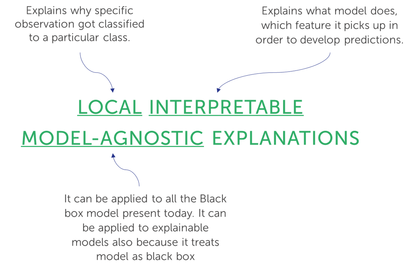
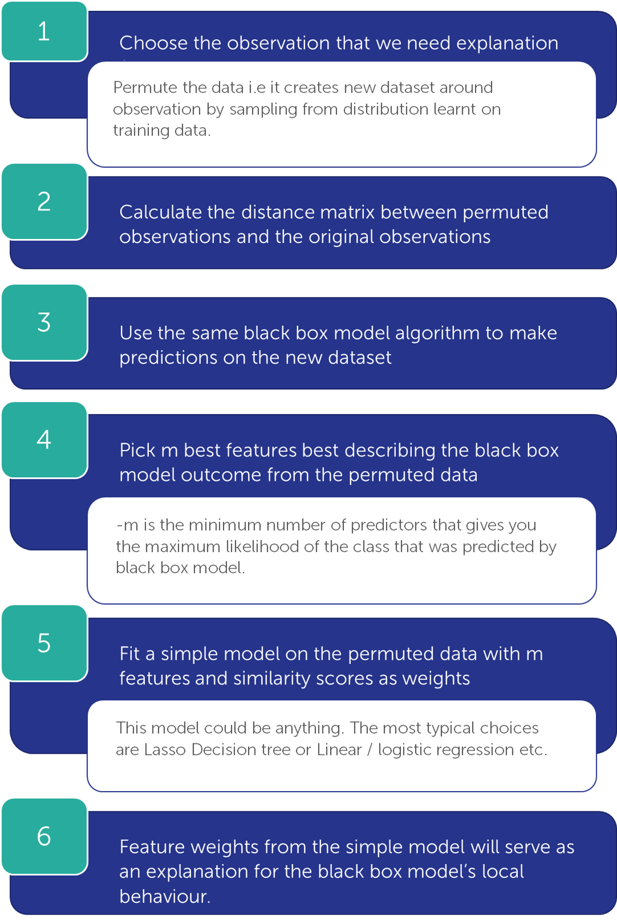
By generating an artificial dataset around the particular observation, we can try to approximate the predictions of Black box model locally using simple interpretable model. Then this model can be served as ‘’local explainer’’ for the Black box model.

However the representation would vary with the type of data. Lime supports Text data, Image data and Tabular type of data:

• For text data: It represents presence or absence of words.
• For image: It represents presence or absence of super pixels
• For tabular data: It is a weighted combination of columns.

This article is focused on tabular data. Tabular data is data that comes in tables, with each row representing an instance and each column a feature.
 

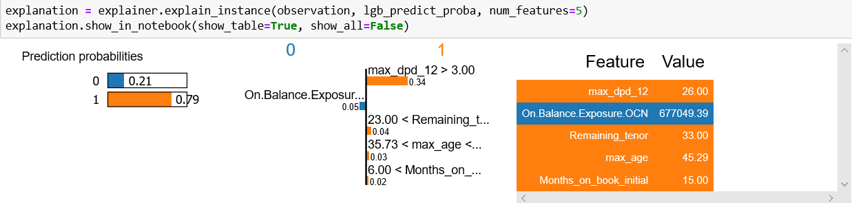
We see that Python gives us output is in 3 parts which can be interpreted as follows:

• The leftmost fig shows that this particular customer has very high (almost 80% ) chance of default.  
• The contribution of each feature to the prediction is denoted just below the feature name in middle fig.
• The table on the right shows the top 4 features(highlighted in orange) that favors class 1 and one feature (highlighted in blue) favors class 0 with actual values of the specific observation

The reliability of this prediction can be given by R²
 

1. LIME can be implemented in Python (packages: lime, Skater) and R (Packages: lime , iml , DALEX). It is very easy to use!
2. Most of these packages are very flexible. You can specify m - the number of features for the model, how you want to permute your data, any simple model that would fit to data. 
3. Furthermore LIME is the interpretation technique that works for tabular, text and image data.
    

1. Fitting of linear model can be inaccurate (but we can check the R squared value to know if it is the case).
2. Lime depends on the random sampling of new points (so it can be unstable).
3. To be extra sure about the model understanding we can make use of SHAP in conjunction with LIME. 
    

The above fig. shows that this particular customer has higher risk of default with the probability of 0.84.  Days past due in past 12 months being higher( 144 days) and On balance exposure also being on the higher side increases his predicted risk of default.
 
The prediction starts from the baseline. The baseline for Shapley values is the average of all predictions. 
Each feature value is a force that either increases or decreases the prediction. Each  feature contributing to push the model output from the base value to the model output.  Features pushing the prediction higher are shown in red, those pushing the prediction lower are in blue.
 

• The method is solidly grounded in mathematics and game theory so we can be certain that it is unbiased  (in the statistical sense) .

• Computational inefficiency. There are 2k possible coalitions for the given number of k factors so depending on the number of variables the analyst must use different level of simplification assumptions. However, on the contrary, SHAP has a fast implementation for tree-based models.

Ceteris paribus is a Latin phrase used to describe the circumstances when we assume aspects other than the one being studied to remain constant.  

In particular, we examine the influence of each explanatory variable, assuming that effects of all other variables are unchanged. Ceteris-paribus (CP) profiles are one-dimensional profiles that examine the curvature across each variable. In essence it shows a conditional expectation of the dependent variable for the particular independent variable  Ceteris-Paribus profiles are also a useful tool for sensitivity analysis.

We can make local diagnostics with CP profiles using Fidelity plot. The idea behind fidelity plots is to select several observations that are closest to the instance of interest. Then, for the selected observations, we plot CP profiles and check how stable they are. Additionally, using actual value of dependent variable for the selected neighbours, we can add residuals to the plot to evaluate the local fit of the model.

1. Identification of neighbors: One can use the similarity measures like Gower similarity measure to identify the neighbors.
2. Calculation and visualization of CP profiles for the selected neighbors: Once nearest neighbors have been identified, we can graphically compare CP profiles for selected (or all) variables. We can say that model predictions are not stable around the instance of interest, if profiles are quite apart from each other and the predictions are stable if we don’t see a large variation for the small changes in the explanatory variables i.e. in nearest neighbors.
3. Analysis of residuals for the neighbors: We can plot the histograms of residuals for the entire dataset. It can give us idea about average performance of the model. 

Local-fidelity plots may be very helpful to check if the model is locally additive and locally stable but for a model with a large number of explanatory variables we may end up with a large number of plots. The drawback is these plots are quite complex and lack objective measures of the quality of the model fit. Thus, they are mainly suitable for an exploratory analysis.

We have arrived at the end of this article. I hope it brings some light to your understanding of LIME, SHAP and CP- Profiles and how can they be used to explain machine learning models. In conclusion: Lime is very good for getting a quick look at what the model does but has consistency issues. Shapley value delivers a full explanation making it it a lot more precise than Lime.

Aside from its practical usefulness, explainability will be ever more crucial for an additional reason: regulators in the European Union and the United States (as well as number of other countries) are pushing more and more boldly for the so-called “right to explanation” which is supposed to, among other things, protect its citizens from gender or race biased decisions when applying for a loan.