The Value-at-Risk metric continues to be widely used in market risk management. This article gives an overview of the current regulatory context of VaR and how is it impacted by the FRTB framework. It also describes where challenges lie in implementation of VaR and the various methodological choices. In addition, associated Value-at-Risk type metrics such as component VaR, incremental VaR and Expected Shortfall are described. Finally, some technical details regarding the Finalyse approach are provided.

Note that while this article refers to VaR, the discussion equally applies to all associate metrics such as component VaR, incremental VaR, weighted VaR, stressed VaR and Expected Shortfall, which are all typically generated using the same model.

Regulatory Context

While VaR is in theory a tool to be used for measurement and management of market risk, in practice, the most common use-case for VaR is to satisfy reporting requirements and for the calculation of regulatory capital for banking institutions using the advanced internal model approach (IMA). Such banks are subject to regulations stemming from the Basel accords, the most relevant being the Fundamental Review of the Trading Book (FRTB) or “Basel IV”. The requirements specified in FRTB can be taken as a best-practice benchmark for all institutions.

IMA requirements arising from adoption of FRTB

FRTB introduces several significant changes from the current framework. The non-quantitative type changes include redefining the scope of the market risk model in terms of banking and trading book, the business level at which risk must be calculated and model usage approved and organisational requirements.

There are multiple quantitative changes introduced by FRTB including the introduction of the Expected Shortfall (ES), minimum standards on data quality and introduction of model performance metrics based on profit and loss attribution, and these three points are briefly discussed below. For full detail, see the official BIS publication and related explanatory notes here [1].

Expected Shortfall

The first notable quantitative changeis the transition from use of VaR and stressed VaR (SVaR) to use of ES as a metric on which regulatory capital is based. Expected shortfall is a measure of the average of all potential losses exceeding VaR at a given confidence interval. The main reason for the transition is that VaR does not capture risks beyond the 99^th percentile and so fails to capture, and disincentivise tail risk. The 97.5^th percentile used in the calculation of ES produces approximately the same value as VaR at the 99^th percentile. Note that back-testing of models remains in terms of VaR and not ES.

Data Standards

The second crucial quantitative change concerns data quality. Banks which use “Historical VaR”, as is becoming more common, are especially dependent on historical data quality. FRTB sets out a risk factor eligibility test which determines whether an observable price/risk factor may be included into the ES model, and in principle could also be applied to a VaR model. Firstly, only “real” prices that are observed can be considered and several criteria can be called upon to determine if a price is real such as if the institution had traded at that price of if a price is available from a vendor. Once the set of real prices have been established the number of observations must exceed a minimum threshold based on the previous 12-month period also considering maximum gap size between consecutive data points and the case of some risk factors which are only observed seasonally.

Trades with risk factors which do not meet these criteria must be passed to a stress-scenario based calculation of capital requirements, with a common stress period. While it is mandatory under IMA to identify such risk factors, it should also be taken as best-practice for non-banking institutions.

P&L attribution

The third substantial quantitative change is the introduction of model performance metrics based on profit-and-loss attribution. The metrics of relevance here are the risk-theoretical P&L (RTPL) ie.. the P&L as predicted by the valuations from the risk management model and associated risk factors, and the Hypothetical P&L (HPL) i.e. the revaluation of the same portfolio over two days excluding effects from intra day events such as fees, further trading etc. Comparing statistical differences in RTPL and HPL will allow for identification of differences between models used in risk management vs. front-office systems. Differences are measured using Spearman correlation and the Kolmogorov-Smirnov test metric, with results mapped into a green, amber or red zone. Trading tests with results falling into the amber zone may continue to use internal models, but are subject to a capital surcharge.

This aspect of model performance measurement is a driver for banking institutions to align pricing systems used by risk departments to those used by the trading desks. It is also a driver to the use of a “full-revaluation” based P&L calculation from a sensitivity based P&L calculation and finally a driver to use common underlying data between risk and FO. As such, it should be seen as best practice by all institutions to use a full-repricing methodology consistent with their front-office systems and to consolidate market data sourcing.

Methodology

Data Quality Methodologies

The most challenging part of a VaR or ES implementation is the sourcing of high-quality input data, and this aspect is of particular importance where simulation scenarios are generated directly from historical data, in which case, a small number of outliers caused by data quality issues can have a material impact on the final VaR or ES number.

Missing data can be treated in several ways depending on the severity of the issue and regulatory rules:

The trade with the associated exposure may be moved out of the VaR or ES model. In the case of FRTB, this induces a regulatory capital add-on. (See details of “Non-modellable Risk Factors” in [1].)
Non-quoted data, such as certain credit spreads for example, may be inferred from prices of quoted market instruments such as bond indices, deposit rates or CDS quotes.
In general, gaps in a risk factor history may be inferred via a data filling model, usually using other similar risk factors as an input, backed up by economic and statistical analysis. Models used here should be frequently recalibrated.
An over-simplified approach, but sometimes observed, is to “flat-fill” the missing data. However, while easy to implement, this approach will severely underestimate the risk.

Any gap filling/proxy methodology itself is a model, requiring validation.

Gaps in a risk factor history may also arise due to removal of data points due to data quality issues for example such as stale or non-liquid quotes, spikes due to operational errors at the time of data sourcing, spikes in equity spot prices due to corporate actions, spikes in rates data due to a sovereign action such as a removal of a currency peg and so on. Risk management may choose to remove such datapoints as these spikes do not reflect the type of risk that the VaR model aims to capture.

It is important that data quality is continuously monitored against an internally documented minimum standard, possibly following that set out in FRTB. Issues with data quality should be automatically flagged to model owners to ensure timely remediation. In the case of FRTB, a deterioration in data quality may lead to loss of internal model approval and associated capital costs.

Simulation Methodology

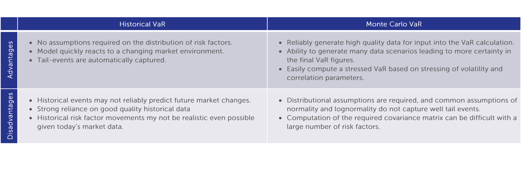
The simulation of changes in risk factors is usually done by either observing historical changes, and applying those to today’s market data, or by computing the covariance of historical changes and generation of simulated changes using a random number generator with an assumption of either a normal or lognormal distribution. The former is referred to as “Historical” VaR, while the latter is referred to as “Monte Carlo” VaR, and similarly for Expected Shortfall.

Within these two main approaches there are several specific advantages, challenges, shortcomings resulting in sources of model risk.

Other assumptions common to both above approaches

For VaR horizons longer than 1-day, for example 20-day, the use of scaling of 1-day changes to hypothetical 20-day changes is sometimes used. A scaling approach is useful in that there is a lower dependency on market data inputs, but it can misrepresent the true distribution of risk-factor changes, underestimating risk as a result. The presence of non-linear payoffs in the portfolio will compound the error. Using actual multi-day changes to generate scenarios avoids any distributional assumptions but will lead to a less available non-overlapping data points which will impact the ability to back-test the model.

As an alternative to scaling of VaR inputs, some institutions will attempt to scale VaR outputs. This is clearly an inferior approach since such scaling will not consider any non-linearity within the portfolio.

A weighted VaR is typically reported alongside VaR, which more recent market events being granted a higher probability of recurring than more distant events. Such weights are typically based on an exponentially weighted moving average. A best practice is to report both weighted and un-weighted VaR or develop a hybrid methodology that is quickly reactive to changing market dynamics but also maintaining non-negligible weights for historical periods of stress.

P&L Calculation Methodology

Full repricing

P&L may be computed by fully revaluing the portfolio on each scenario path and subtracting the current portfolio value. This approach will naturally produce an accurate P&L on each path but is usually only feasible where a lower number of paths are used such as in Historical VaR and where closed-form/analytical pricing is available. A full revaluation approach requires that the risk department has access to pricing models, and ideally that those models and all market data inputs are aligned with front-office systems to ensure that risk department outputs truly reflect the risk within the trading book. See the P&L attribution metrics introduced within FRTB.

Sensitivity Based Approach

Another approach is to model the P&L change by determining in advance the sensitivity to risk factor changes and cross-sensitivities to simultaneous risk factor changes. Assuming sensitivities are available analytically, this solution is much quicker than full revaluation but typically excludes certain higher order risks and can be difficult for products with many sensitivities such as basket equity options for example. This solution could be taken as a fall-back to full repricing in cases where analytic pricing is not available. Again, sensitivities will need to be computed by the risk department requiring the need for pricing models, or alternatively may be sourced from front-office.

VaR and associated metrics

An intermediate output of any VaR or ES application is a set of simulated P&L vectors at trade level. VaR applications will typically allow the user to aggregate P&Ls along various dimensions i.e. desk/business/asset class levels in addition to reporting the overall portfolio VaR. VaR reported at any sub-level, but typically at individual trade level, is known as Standalone VaR and represents the undiversified risk coming from the trade positions at that level. Unlike P&L, standalone VaRs will not sum to the VaR of the overall portfolio as the diversification benefit due to hedging of positions is not captured. In fact, the difference between sum of standalone VaRs, possibly at the business level, and the overall portfolio VaR may be a measure of diversification benefit.

An alternative trade level metric which takes diversification into account, and whose sum is the portfolio VaR is known as Component-VaR (CVaR). Unlike VaR, CVaR can be positive and negative, and the sign reflects the offsetting nature of trades/asset classes within a portfolio hedge each other. For example, equity and rates portfolios will have CVaRs of opposite sign typically. A commonly used approach to CVaR calculation is the kernel estimation methodology described in [2]. There are some caveats to be considered in using CVaR: CVaR is a mathematical construct – it does not tell you the contribution a trade has to the overall VaR, rather it is an indicator to the direction of hedging and the relative contribution to VaR hedging benefit from a trade. CVaR tends to be useful mostly for trades associated with risk factors which are the driving factors behind a portfolio’s P&L. CVaR from trades associated with other risk factors tend to be noisy and so difficult to interpret. Finally, due to the requirement that sum of CVaRs is equal to the overall portfolio VaR a scaling factor is used in the CVaR calculation. In cases where a portfolio is well hedged this scaling factor can dramatically inflate CVaR values causing the magnitude of the CVaR value to lose any economic interpretation. For example, in an extreme situation, a portfolio that is almost perfectly hedged can have CVaRs approaching infinity. In conclusion, CVaR figures should be taken as indicators and not be used as an input to risk limits or inputs to other models.

Incremental VaR is simply the difference in portfolio VaR with and without a given trade. Like VaR, the sum of incremental VaRs does not sum to the overall VaR. Incremental VaR may be used for pre-trade analysis for example.

Another commonly seen metrics is Stressed VaR. Stressed VaR is simply VaR but calibrated to a period of historical stress. The challenge with stressed VaR is in determining which historical period to use, since current regulatory requirements specify that the period to used is the one that maximises the VaR value. In theory it is not possible to know this without computing VaR on every historical period, and so in practice in industry models are employed to answer this question. Another challenge with stressed VaR is availability of historical data. Note that under FRTB, VaR and Stressed-VaR are replaced with a single Expected Shortfall metric that is calibrated to a period of significant market stress.

Weighted VaR is like VaR except that in simulations a greater probability is assigned to more recent market behaviour. For example, if the market suddenly experiences a volatile period, the simulation of risk factors quickly adjusts resulting in larger simulated shocks. This allows VaR to be reactive and captures real-world features such as volatility clustering but may diminish extreme events further into the past which should still be considered. In addition, having a low weight applying to the most distant historical observation ensures that the removal of that last point in the rolling historical observation windows does not cause a jump in VaR. It is common that either both VaR and weighted VaR are both reported, or a hybrid methodology is used, essentially taking the worst of VaR and weighted VaR.

FRTB introduces the Expected Shortfall (ES) as the standard measure of market risk, replacing VaR and stressed-VaR in the internal model approach (IMA). A benefit of ES is that it is sub-additive i.e. that it will correctly capture diversification benefit. ES is the average of losses beyond a given percentile, and so will capture extreme events that are missed by VaR.

All the above metrics are easily computable for the P&L vector output from any simulation engine. Once P&Ls are available the only remaining decision will be the level (levels) of aggregation. Ideally all VaR at any level of aggregation i.e. trade/desk/business, or at product level or risk factor level should be available. The granularity available will depend on the VaR methodology being used, for example, a sensitivity based P&L will naturally allow P&Ls from certain risk factor types to be easily segregated and the resulting VaR determined, whereas in a full repricing approach, changes in all risk factors are simultaneously used and so risk factor level granularity is not an immediate output. Therefore, risk reporting requirements should be considered at the outset of choosing the VaR methodology.

Model Risk and Model Testing

There are multiple sources of model risk within VaR models and sub-models such as data enhancement models and pricing models.

Within data enhancement models the obvious risk in parameter estimation is present, and in pricing models the risk due to any pricing approximations needs to be considered. Risk exists where the risk factors being simulated do not correspond directly to the data needed for pricing; for example where only a small number of tenors on an interest rate curve are simulated instead of the full curve. Risk exists where there is a dependence on non-observable market factors, in which case models may be used to infer the required data from observable market data, and a similar problem arises when there is a dependency on market factors which do not have a history.

Within VaR itself, estimation error exists in the construction of the covariance matrix needed for Monte Carlo VaR, and intrinsically in historical VaR since the observed history is of course only a sample from the real-world distribution of that risk factor. Risk will exist in any VaR scaling methodologies used, and in the choice of weighting. Risk will exist in the choice of number of simulation paths in Monte Carlo VaR where a lower number of paths can give risk to uncertainty in VaR itself. Aside from risk coming from the mathematical aspects, further risk may be due to coding implementation, correctness of trade data, scope control and alignment with regulatory requirements.

In the case of the non-mathematical aspects, risk may be mitigated through good governance, controls and a model validation and audit framework. In the case of the model risk due to the mathematical aspects, a back-testing framework has been the standard approach in which a periodic assessment is made of the correspondence of the historically observed P&Ls, both actual and hypothetical vs. the frequency of occurrence of the P&Ls which exceed the VaR level. For example, a 99% VaR, which should be tested as part of FRTB, is intended to represent the loss the portfolio would only exceed one day in one hundred, on average.

It is natural to see a few exceptions over the 250 day backtesting window, but a larger number of exceptions that can’t be explained by non-modellable risk factors may indicate missing risk within the model. The FRTB framework quantifies the allowable number of exceptions, and thresholds which indicate poor model performance and model failure, with increasing levels of capital requirements or possible withdrawal of model approval. In the case that the model no longer meets the backtesting requirements a fallback to the FRTB standardised approach is used.

Other than backtesting, P&L attribution tests are also introduced within FRTB as discussed above.

Implementation Details at Finalyse

This section describes the Finalyse implementation, a close reflection of industry’s best standard.

Market Data

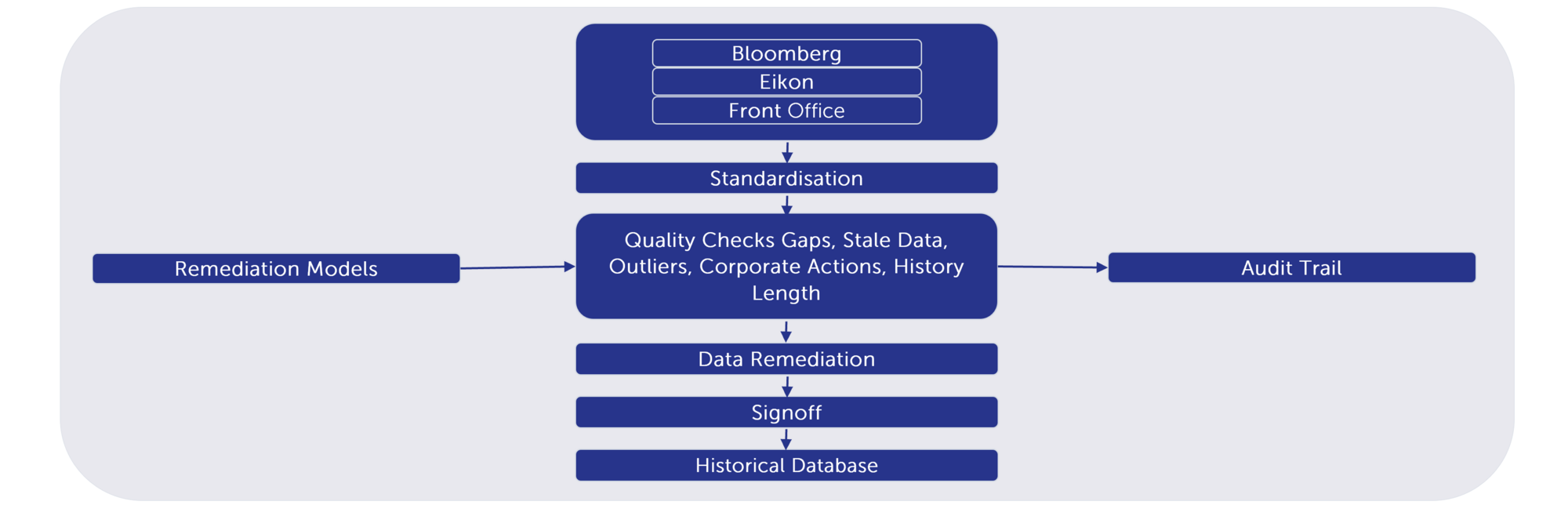
Market data typically comes from several sources which need to be reliable and consistent. As with all data sources it needs to first be standardised into a format which the coding libraries can access. Afterward a data quality pipeline performs data quality checks, data enhancement and calculation of historical changes for each risk factor.

Pricing and Simulation

Almost all pricing libraries today follow an object orientated approach. Typically, this is a C++ library as a base, with interfaces for Excel or Python. In Finalyse we use Python to manage all aspects of VaR calculation except pricing.

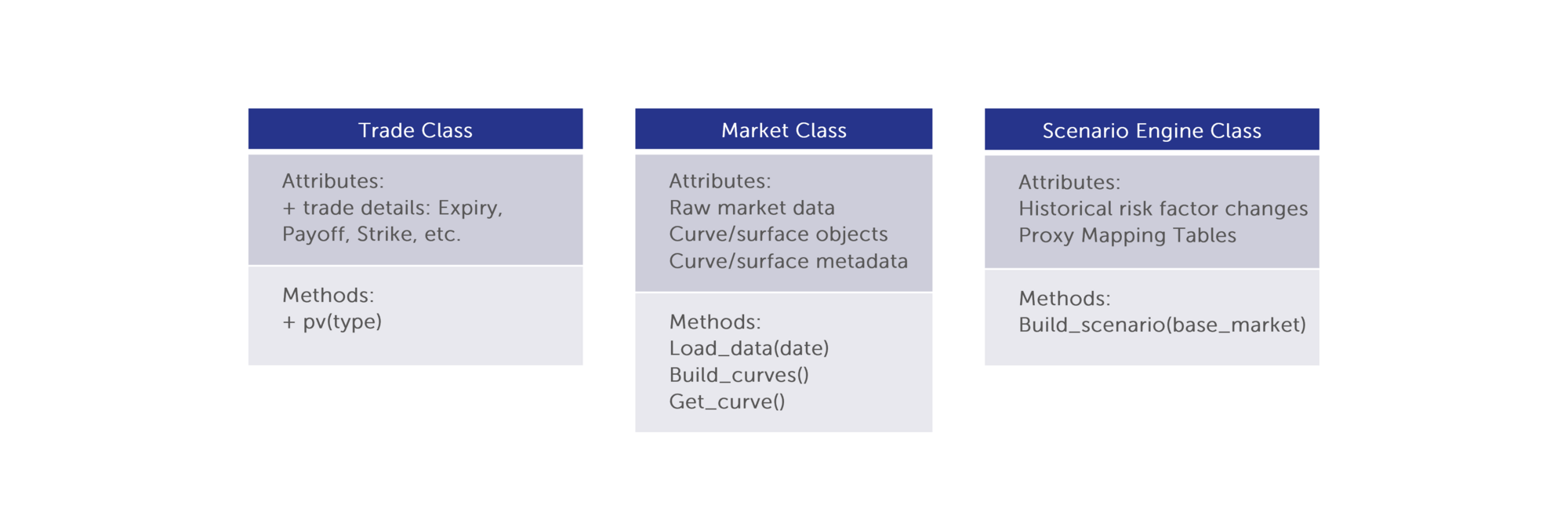
In the UML diagram below, an instance of the Trade Class is responsible for holding all payoff information. It knows which pricing library to use and invokes that library when the value of the trade is requested. Instances of the trade class are built from the trade data files.

Secondly, an instance of the Market Class holds all market information on a given day. It also holds “curve” and “surface” objects which may be passed to the trade instance as needed for pricing. The market instance builds these objects as needed (lazy evaluation). The market class is responsible for parsing data from the various sources and building it into a coherent data set which all other classes may then use, for example, the scenario engine class.

The Scenario Engine Class reads historical market data from the pipeline described above and reads today’s market data from an instance of the market class. Information on what risk factors are required is passed from the set of trade instances. The scenario engine then builds required scenarios either based on historical or Monte Carlo VaR or a stress test design, and creates new market instances, one per scenario. In the case of Monte Carlo VaR the Finalyse solution captures heavy tails following the approach used in [3]. Furthermore, the solution avoids the step of covariance matrix construction following the approach used in [4]. The portfolio is then priced using each of these market instances to determine the P&L distribution. Instances of the scenario engine may also be used to represent a stress test, and so stress testing fits naturally into the VaR application.

Reporting

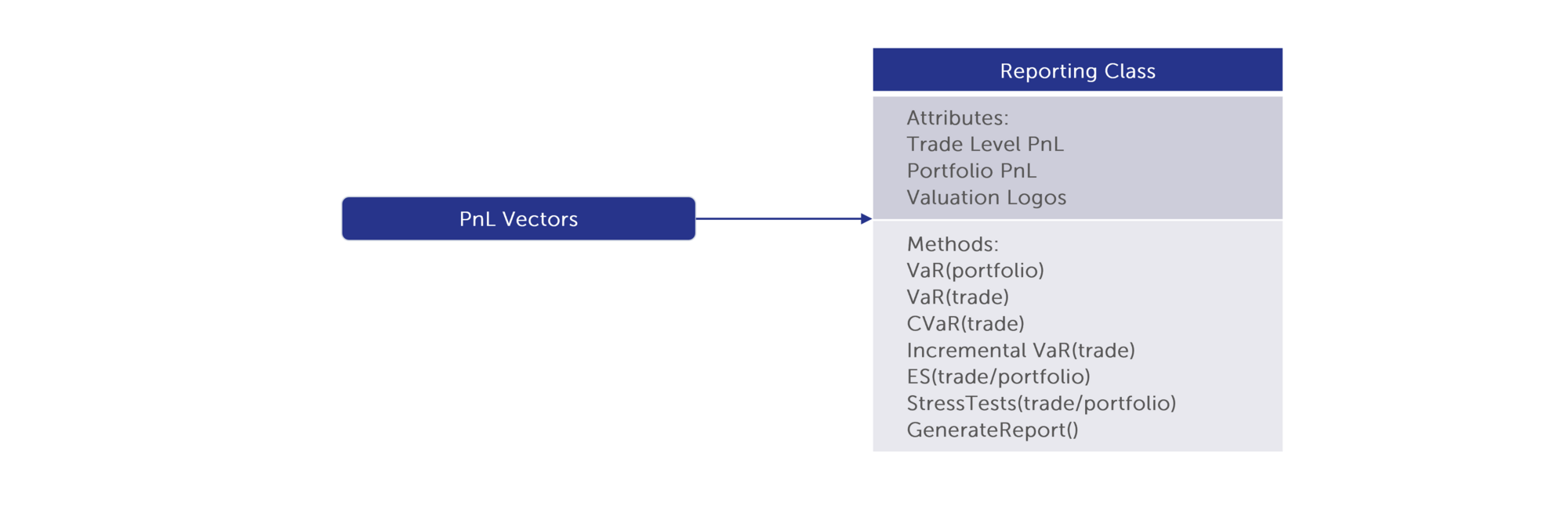
Calculation of the various VaR metrics is straightforward once the P&Ls are known from each scenario. A reporting class is used to complete this task, and present the results and statistics such as CVaR, incremental VaR, ES etc. at the needed aggregation level as described in the previous text.

Conclusion

While VaR is an old concept it continues to be relevant today as a method to determine regulatory capital and as an easy-to-interpret metric that can be applied to any asset class and by any institution.

Conceptually VaR is a simple methodology and there are many choices when it comes to implementation. The driving factors in this choice are typically regulatory and reporting requirements. For risk management, the focus should be on mitigating model risk. There are several sources of model risk, the most obvious being quality of historical data. Care should be taken to implement a sound governance framework to ensure:

Consistency of data quality ongoing monitoring,
The alignment of pricing models between middle and front office,
The soundness of the implementation and appropriateness of methodological choices via model validation and audit,
The ongoing performance of the model via back-testing and pricing reconciliation,
The quality of documentation,
And most importantly, the compliance with regulatory requirements.

Bibliography

Basel Committee on Banking Supervision, “Minimum capital requirements for market risk,” 14 January 2019. [Online]. Available: https://www.bis.org/bcbs/publ/d457.htm
E. &. Smillie, “Cracking VaR with kernels,” Risk, pp. 70-74, August 2006.
S. Mandan, “The Variance Gamma Model for Share Market Returns,” The Journal of Business, vol. 63, no. 4, pp. 511-524, 1990.
RiskMetrics, “Monte Carlo Simulation using the Benson-Zangari Approach,” 2013.

Share this article:

Looking to remain up-to-date with regulatory requirements?

Table of contents

Related Articles