The EBA proposes to allow the model differentiation sample to be not representative of the application portfolio. The CRR mandates that the dataset used for model development is representative of the institution’s actual population of obligors or exposures. This requirement has been repeated in the EBA guidelines for PD and LGD estimation.
The recent paper on CCF guidelines introduced a more flexible framework for representativeness, allowing the risk differentiation sample to exhibit a lack of representativeness from the application portfolio, as long this doesn’t affect the model performance.
Such flexibility is particularly relevant for low default portfolios (LDP) for which there is a high class imbalance. Such portfolios are a challenge for traditional statistical models as it is possible to get a high accuracy by simply always predicting the absence of default, hence preventing the model to correctly discriminate between defaulting and non-defaulting obligors. By relaxing the need for representativeness with the application portfolio in the modelling phase, the EBA allows the use of data resampling techniques such oversampling, undersampling or more advanced synthetic data generation techniques.
The EBA considers simplifying the modelling of MoC A/B by adding a fallback approach. The modelling of Margin of Conservatism (MoC) is inherently complex. MoCs need to be proportional to the “expected range of estimation errors”, and to the existing data issues. For the usual MoC (type A) calibration, MoC calibration consists of 1) estimating the amount of data points affected by a certain deficiency and 2) estimating an appropriately conservative amount of by which these data should be stressed. These stressed datapoints are introduced to the calibration sample and the model is recalibrated on this stressed dataset.
While there could be some meaningful simplification in step 2), which will be proposed in the following paragraph, the complexity in step 1) is inescapable. There are no heuristics available to conservatively estimate the amount of data points affected by e.g. a change in the definition of default. Due to the absence of a natural upper bound (beyond the 100% limit) for the affected data, the first step of the MoC calculation cannot be simplified through conventional modeling techniques.
For step 2), a simplification is possible. The ratio of modelling effort to impact is the highest when many different issues are identified that each only affect a small number of data points. As the Guidelines for PD and LGD Estimation already allow for the joint quantification of deficiencies, a meaningful simplification could be to simply add the number of affected data points selected for the IRB Simplified approach, and assigning the maximum realized LGD of 100%, or CCF of 100%, etc. In formula form:
$$MoC_{\text{simplified}} = \begin{array}{c} \#\text{Selected data points} \\ \hline \#\text{Total data points in RDS} \end{array}$$
Then the simplified MoC is simply added (instead of multiplied) to the final risk parameter. For example for PD:
$$PD_{\text{final}} = PD \cdot (MoC_{A} + MoC_{B} + MoC_{C}) + MoC_{\text{simplified}}$$
Consider an example RDS for which 0.03% of datapoints have a wide variety of issues. For some the risk drivers are unreliable, for some the default status is uncertain. The most conservative impact that these data points could have would be for each of them to be counted as a default in the calibration, where they would weight for at most 0.03% of the total segment. Therefore adding 0.03% to each of the grades is a sufficiently conservative and simple fallback option.
The EBA considers standardizing the MoC C approach to address high level of heterogeneity among institutions, as well as issues with low default portfolios. Institutions use different approaches when it comes to MoC category C, set at different levels of conservatism. Organizations would benefit significantly if the EBA were to standardize supervisory expectations by adopting a bootstrapping-based methodology. Additionally, there are multiple industry standard values at which the confidence level is set. Providing additional guidance on how this confidence level for MoC C quantification should be set could bring clarity to banks.
The EBA proposes an absolute or percentage based fallback approach to estimate (in)direct costs. The direct costs, which are costs directly related to a default e.g., fees due to the foreclosure of a house, and indirect costs, which are the costs of maintaining the department that manages non-performing loans, are part of the realized LGD.
An inflation indexed absolute value would be the most appropriate for the direct costs, as direct costs do not scale with LGD. This absolute amount should be set to a conservative figure by the EBA or the national competent authority to ensure they reflect reality conservatively.
For the indirect costs an absolute value that is dependent on the size of the portfolio or the size of the institution would be sensible. As before, the EBA or national competent authorities should set the number in a conservative manner.
EBA proposes to allow a simplified DT LGD adjustment. The downturn adjustment for LGD involves a complicated modelling exercise. There are 3 methods laid out in the RTS on downturn estimation, and the most risk sensitive method requires banks to “model appropriately the loss components materially affected by the downturn period under consideration”. The loss components are: realised LGDs, decreased annual recoveries, decreased number of cures and prolonged time in default. Modelling these 4 dimensions is already a significant challenge, potential simplifications are discussed below.
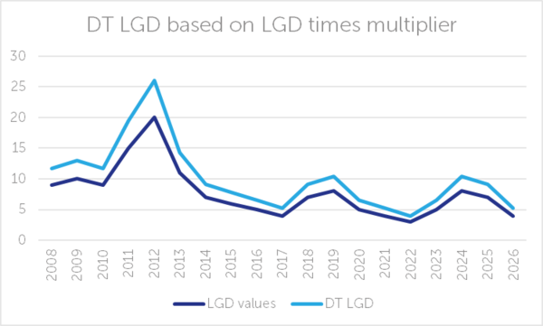
An intuitive but highly cyclical approach to simplified DT LGD modelling is to multiply the LGD parameter by some fixed constant, for instance a constant based on the LRA LGD and the reference value (the average realized LGD in the worst two years observed). This method leads to a DT LGD that is even more cyclical than the underlying LGD model, as visualized below in Figure 1. Cyclicality in the DT LGD leads to systemic risk since in a downturn of the credit cycle it leads to higher capital requirements for all institutions at exactly the most difficult time to raise capital. Paragraph 17 of the EBA Guidelines on DT estimation specifies that “institutions should apply an adjustment to their downturn LGD estimates to limit the capital impact of an economic downturn”.
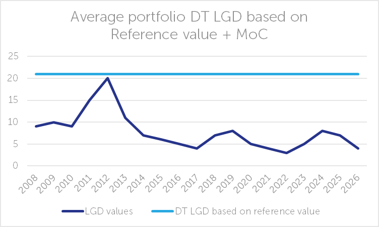
A more countercyclical way, and therefore preferred way, to introduce a simplified DT LGD regime is to multiply the LGD model with a scalar that changes every month as a function of the average model LGD of the portfolio such that the average DT LGD stays the same on portfolio level. The constant is calculated each month as the reference value divided by the portfolio level average model LGD of that month. In formula form:
$$LGD_{DT} = LGD_{i} \cdot \begin{array}{c} \text{Reference value} \\ \hline \text{Average portfolio LGD for given month t} \end{array} \cdot MoC$$
\(\text{Reference value} =\) average realized LGD of the worst 2 years in the historical observation period, a number that remains fixed after model development.
\(\text{Average portfolio LGD} =\) the average output of the LGD model on portfolio level for the given reporting month.
\(LGD_{i} =\) is the LGD for facility i.
While the DT LGD value would be different for facilities in different pools (there is still risk discrimination on the pool level), the portfolio level average DT LGD would remain constant. This is the extreme end of through the cycle modelling (see Figure 2). Note that a consequence of this method is that the pool level DT LGD would be different from reporting date to reporting date.
If this method is deemed not conservative enough compared to the risk sensitive IRB models the reference value can also be further increased with a supervisory add on.
The EBA proposes a SA-like approach for the estimation of LGD in default. The SA risk weight for defaults is 150% or 100% depending on the specific credit risk adjustments. Meanwhile the risk weight for defaulted exposures in IRB approach is equal to:
$$Risk\ Weight = Max(0, 12.5(DT\ LGD - ELBE\ LGD)).$$
Where ELBE (expected loss best estimate) LGD is the LGD in default without the DT adjustment, MoC or any other unexpected loss adjustment. Note that if the difference between the DT LGD and ELBE equals 8 %, the IRB risk weights are already comparable to the standardized regime for defaulted assets. An SA-like approach for RWA calculation of the defaulted exposures would significantly reduce the complexity of modelling, and the standardized risk weights are not overly punitive.
In this discussion paper, the EBA argues that in general CCF models have low discriminatory power, a fact that is also underlined by academic research on the topic. See for example Thakman & Ma (2017). There are however controversies regarding the appropriateness of alternative methods (see Gürtler, Hibbeln & Usselmann (2018)) This low predictive ability can stem from several reasons, including (among others) drawing patterns across different facilities for a given obligor, the extreme variability of the observations near the region of instability, the pre-default changes in limits and the presence of post default drawings.
This lack of discriminatory power, coupled with the floor at 50% of the SA-CCF value and the applicability of the CCF IRB to only revolving exposures, implies a very limited gain in terms of risk sensitivity, defeating one of the major goals of the IRB approach (EBA/DP/2015/01). Therefore, the marginal risk sensitivity gains of the IRB approach might not be justified in terms of the burden of CCF modelling and the EBA proposes to extend the fixed IRB-CCF derogation proposed in the consultation paper on CCF modelling. This would allow for the optional use of fixed CCF for all exposures while still using the IRB approach.
This option is indeed a simplification in the sense that it overcomes the burden of developing and maintaining an appropriate CCF model, but it would be costlier in terms of RWA. Under the fixed CCF, banks should apply an MoC such that the CCF has a minimum value of 100%, and when backtesting shows realized CCF values above 100%, the MoC should be raised in order to keep the parameter’s conservativeness.
EBA proposes to allow cohort approaches for IRB CCF modelling. Article 182(1)(g) specifies that “institutions’ IRB-CCF shall be estimated using a 12-month fixed-horizon approach”. Such requirement follows the Basel 3 framework prescriptions (CRE 36.93) regarding the CCF measurement.
Such approach has its inherent limitations and could lead to biases. First, a 12-month fixed window implies that there are observations, called “fast defaults”, for which there are no risk drivers observed 12 months before the default because the default occurred less than 12 months after origination. Those observations can either be excluded from the modelling sample or can be included with the risk drivers’ values at origination. In both cases, this could distort the model accuracy. For risk quantification, all observations, including fast defaults, should be included. Such fast default observations’ impact on the LRA should be estimated and potentially mitigated with MoC to overcome any undue influence. Additionally, the use of a fixed window period will prevent capturing seasonal variations within the 12 month window.
To mitigate those biases, the EBA proposes in this discussion paper to allow for the use of a cohort approach. Such an approach would reduce the biases mentioned earlier by including all the observations and potentially ensuring consistency with the cohort approach allowed for the PD. It would however introduce new biases by mixing observations with different horizons and by setting a fixed start of cohort date. Unlike the current backward-looking approach (where seasonality averages out across default dates) a forward-looking cohort approach relies on a specific starting date. If undrawn amounts or risk drivers are seasonal, this single snapshot may not accurately represent their year-round distribution. Furthermore, the use of the cohort approach should be justified: any significant deviation in the LRA obtained with the cohort approach with respect to the LRA CCF calculated according to the 12-month fixed window approach should be explained. Far from simplifying the CCF IRB modelling approach, this increases the complexity and the burden of the modeler by obliging them to use both approaches and quantify the differences. This introduces additional uncertainty and variability for CCF estimates, as there are no standardized definitions for significant deviations or the justifications required to support them.
Are you looking to simplify your IRB model landscape? To put a stop to the sprawling repair programs and countless findings? Drawing on extensive experience with supervisory engagements, Finalyse can support banks in their IRB and standardized journey.
Finalyse has successfully helped clients:
Our consultants bring hands-on experience across regulatory, risk, and operational dimensions of credit risk, enabling institutions to move from concept to execution with confidence.
EBA is proposing the introduction of impactful simplifications for IRB CCF as well as the introduction of a simplified IRB approach.
The simplified IRB approach could provide a significant decrease of the modelling complexity, thereby reducing findings and add-ons going forward.
When these significant simplifications become guidance it could lead to the forced redevelopment of IRB models, for instance because a bank was currently using some exceptional arrangement that gets scrapped due to simplifications.
Finalyse InsuranceFinalyse offers specialized consulting for insurance and pension sectors, focusing on risk management, actuarial modeling, and regulatory compliance. Their services include Solvency II support, IFRS 17 implementation, and climate risk assessments, ensuring robust frameworks and regulatory alignment for institutions. |

Check out Finalyse Insurance services list that could help your business.
Get to know the people behind our services, feel free to ask them any questions.
Read Finalyse client cases regarding our insurance service offer.
Read Finalyse blog articles regarding our insurance service offer.
Designed to meet regulatory and strategic requirements of the Actuarial and Risk department
Designed to meet regulatory and strategic requirements of the Actuarial and Risk department.
Designed to provide cost-efficient and independent assurance to insurance and reinsurance undertakings
Finalyse BankingFinalyse leverages 35+ years of banking expertise to guide you through regulatory challenges with tailored risk solutions. |

Designed to help your Risk Management (Validation/AI Team) department in complying with EU AI Act regulatory requirements
A tool for banks to validate the implementation of RWA calculations and be better prepared for CRR3 in 2025
In 2027, FRTB will become the European norm for Pillar I market risk. Enhanced reporting requirements will also kick in at the start of the year. Are you on track?
Finalyse ValuationValuing complex products is both costly and demanding, requiring quality data, advanced models, and expert support. Finalyse Valuation Services are tailored to client needs, ensuring transparency and ongoing collaboration. Our experts analyse and reconcile counterparty prices to explain and document any differences. |

Helping clients to reconcile price disputes
Save time reviewing the reports instead of producing them yourself
Helping institutions to cope with reporting-related requirements
Be confident about your derivative values with holistic market data at hand
Finalyse PublicationsDiscover Finalyse writings, written for you by our experienced consultants, read whitepapers, our RegBrief and blog articles to stay ahead of the trends in the Banking, Insurance and Managed Services world |

Finalyse’s take on risk-mitigation techniques and the regulatory requirements that they address
A regularly updated catalogue of key financial policy changes, focusing on risk management, reporting, governance, accounting, and trading
Read Finalyse whitepapers and research materials on trending subjects
About FinalyseOur aim is to support our clients incorporating changes and innovations in valuation, risk and compliance. We share the ambition to contribute to a sustainable and resilient financial system. Facing these extraordinary challenges is what drives us every day. |

Finalyse CareersUnlock your potential with Finalyse: as risk management pioneers with over 35 years of experience, we provide advisory services and empower clients in making informed decisions. Our mission is to support them in adapting to changes and innovations, contributing to a sustainable and resilient financial system. |

Get to know our diverse and multicultural teams, committed to bring new ideas
We combine growing fintech expertise, ownership, and a passion for tailored solutions to make a real impact
Discover our three business lines and the expert teams delivering smart, reliable support