


Augustin de Maere is a Principal Consultant based in Finalyse Brussels, leading the Market Risk & ALM practice with François-Xavier Duqué, with a specific focus on Interest Rate Risk and Economic Capital modelling. He has been involved in the development or validation of several interest rate models, covering all the aspects of the model chain, from interest rate scenario generators to the calibration of behavioural models (non-maturity deposits, …) and the building of portfolio revaluation engine.
Non-maturity deposits are liabilities that are characterized by two key features: the interest-rate paid on the liability is set up unilaterally by the Bank, and customer is free to withdraw the funds at any point in time. The contractual maturity is therefore overnight, but in practice, these liabilities are known to exhibit a significant stickiness, and most have a significant effective duration.
The behaviour of the balances may be modelled under three different regimes: in run-off, in a static balance-sheet and assuming inflows of new clients. The treatment of non-maturity deposits is therefore at the edge between liquidity management and asset & liability management. It is important for banks to properly capture these features, because it will result in a more accurate assessment of their liquidity needs and interest-rate sensitivities. It will also play a crucial role in the transfer pricing of deposits, the interest-rate risk in the banking book calculations (IRRBB) and the internal liquidity adequacy assessment process (ILAAP).
The factors affecting non-maturity deposits can be classified in three different types:
Modelling non-maturity deposits consists in correctly capturing the relationship between the client rate and balances with the prevailing market rates. The prevailing market rates are usually swap rates, government bond rates or central bank interest rates. These rates are assumed to reflect the risk-free yield a bank may expect from its assets.
Three levels of models are therefore required, as illustrated in Figure 1. A first model will capture the evolution of market rates. A second model will forecast the evolution of the deposit rates conditional on these market rates. Finally, a third model will provide the change in volumes. The next sections will provide more insights in the modelling requirements and the most common difficulties encountered in the development of these models.
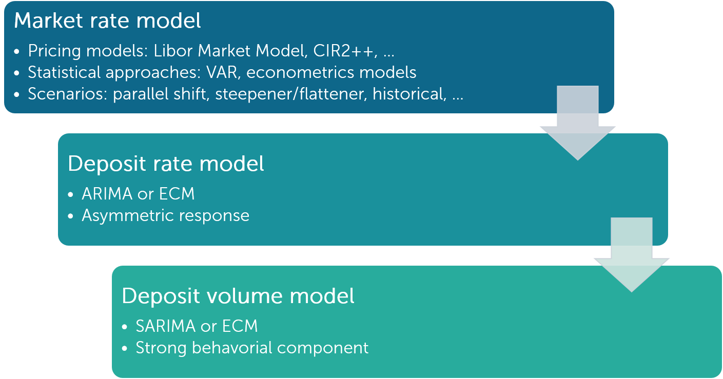
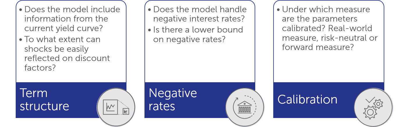
Market models are usually pricing models, such as the 2-factor Cox-Ingersoll-Ross model (CIR2++) or the Libor Market Model (LMM). These models are usually calibrated on the current interest rate swap curve and a volatility surface from interest rate derivatives (e.g. swaptions). Some important properties of these models that the bank should be aware are highlighted in Figure 2.
With statistical models, the aim is to forecast the future volatility of interest rates based on the past. The simplest approach is to apply a vector autoregressive (VAR) model to the principal components of the yield curve, but more advanced approaches may also be considered, e.g. by incorporating econometric expertise and linking the projections to macro-economic factors or by using machine learning models such as long short-term memory (LTSM) neural networks.
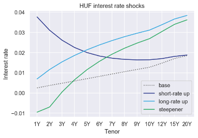
Finally, the evolution of the market rates is sometimes simply directly provided by the Bank or by the regulator. For instance, the European Banking Authority (EBA) prescribes specific interest rate shocks in its most recent Interest Rate Risk in the Banking Book guidelines (IRRBB). Some of these shocks are reported in Figure 3.
All these approaches have their advantages and shortcomings, and Banks will typically rely on one or more approaches at this level. For instance, a risk-neutral model may be used for the valuation of the NMD, an econometric model for the budget planning, and expert scenarios in the context of interest rate risk in the banking book capital calculations. If several yield curves are used by a bank, a specific care should be taken for the modelling of the basis between these curves.
The second step consists in modelling the interest rates paid on the deposits as a function of the interest rates prevailing on the market. A first technical challenge however resides in the statistical properties of the market rates:
The correlation issue can be solved by relying on principal component analysis (PCA). PCA is a data analysis technique to transform a set of correlated observations into uncorrelated variables. These uncorrelated variables are then classified by the amount of the explained variance, and usually, only a few principal components are sufficient to explain most of the observed variance.
What is Principal Component Analysis?
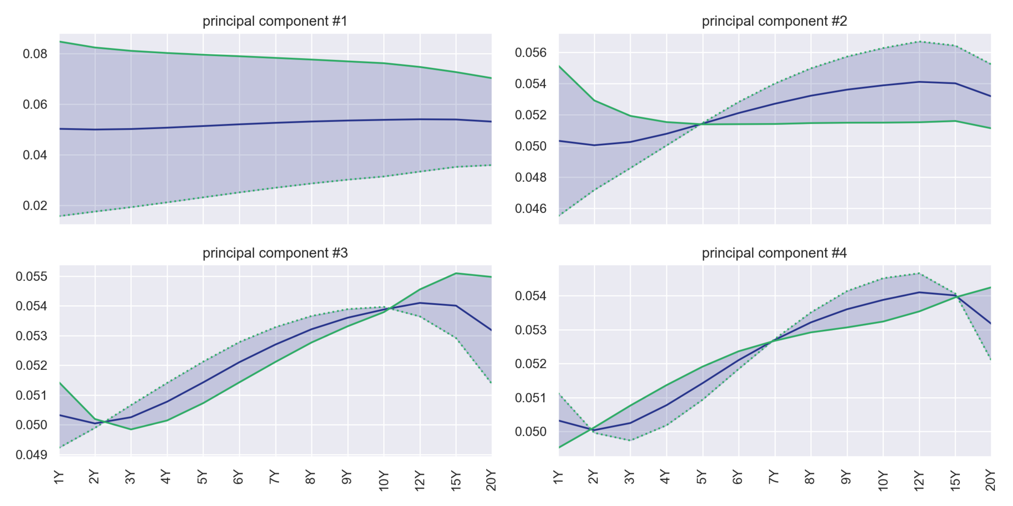
Principal Component Analysis is a dimensionality reduction technique, which aims at transforming a set of correlated observations into uncorrelated variables. If \(y_T (t)\) denote the tenor \(T\) of the swap curve at time \(t\), then the curve can be decomposed as a sum of basic curves \(v_(i,T)\) called principal components:
$$y_T(t) = \sum_{i=1}^{N} a_i(t)\, v_{i,T} \approx \sum_{i=1}^{4} a_i(t)\, v_{i,T}$$
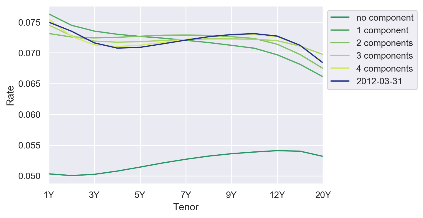
The weights \(a_i (t)\) applied to each principal component are the factor loadings. There are as many principal components as there are variables, but usually, only the most significant principal components are extracted.
The PCA has therefore two key advantages in general:
In the case of yield curve modelling, two other side benefits of PCA arise:
Like market rates, both time series also appear to have a unit-root, and specific regression techniques have therefore to be used. The most standard technique for unit-root process are ARIMA process: the time series is first differentiated until it becomes stationary and is then regressed against stationary exogenous variables \(Xt\). For the deposit rate \(rt\), the model formulation could be:
$$ \Delta r_t = \alpha \Delta r_{t-1} + \beta X_t + \gamma + \epsilon_t $$
In the above equation, the exogenous variables are stationary, which implies that each variable must be differentiated until it becomes stationary. While this formulation is extremely flexible and provides excellent one-step ahead projections, its long-term stability may be deteriorated, because it does not include the fact that there is a long-term equilibrium between the deposit rates and the market rates. This long-term equilibrium is captured in a cointegration relationship: while deposit rates and market rates may have a unit-root, there is a linear combination of these variables that is stationary, and this combination can be exploited in an Error Correction Model (ECM). If \(Xt(ex)\) and \(Xt(co)\) are respectively the stationary and non-stationary exogenous variables, the deposit rate is modelled as:
$$ \Delta r_t = \alpha \left(r_{t-1} - \eta X_{t-1}^{co}\right) + D X_t^{ex} + \gamma + \epsilon_t $$
The term in parenthesis represent the long-term trend for the deposit rate \(rt\). Assuming that \(α\)<0, the process will tend to converge exponentially fast toward the long-term equilibrium value of \(η X(t-1)(co) (a)\). However, the short-term dynamic will be perturbed by shocks arising from other stationary short-term variables in \(D Xt(ex) \)and from the other unexplained factors \(ϵt\).
As an illustration, two models of the national average of deposit rates for overnight and time deposits were calibrated using the error correction model formulation. The models were assessed not only for their one-step ahead statistical properties (Bayesian Information Criterion, t-tests on significance, ADF and KPSS tests for stationarity, Ljung-Box tests for autocorrelation of the residuals, …) but also for their economic soundness and the quality of their out-of-sample predictions (starting from December 2007). In an out-of-sample prediction, the predictions of the model at a given time step are given as input for the forecast of the next time step, and so on, therefore ensuring that the evolution of the model is significantly driven by the exogenous factors, and not only by its auto-regressive properties.
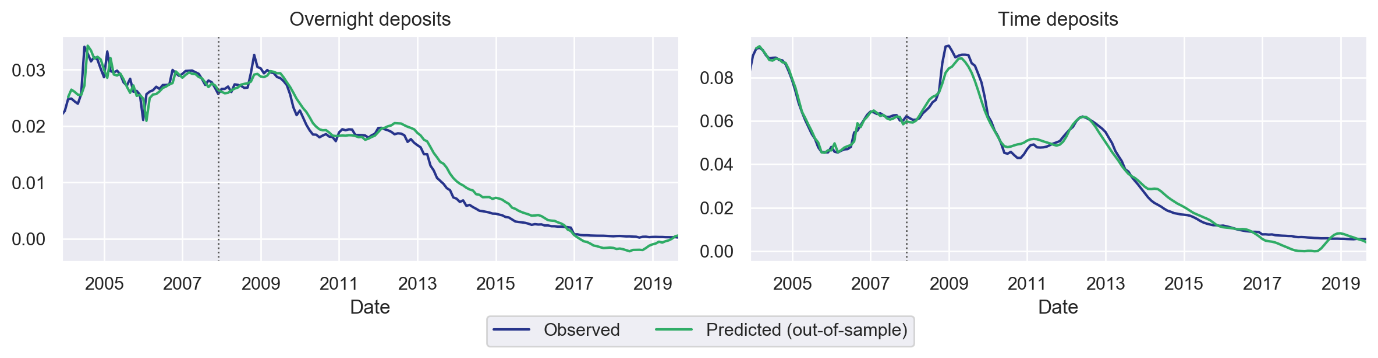
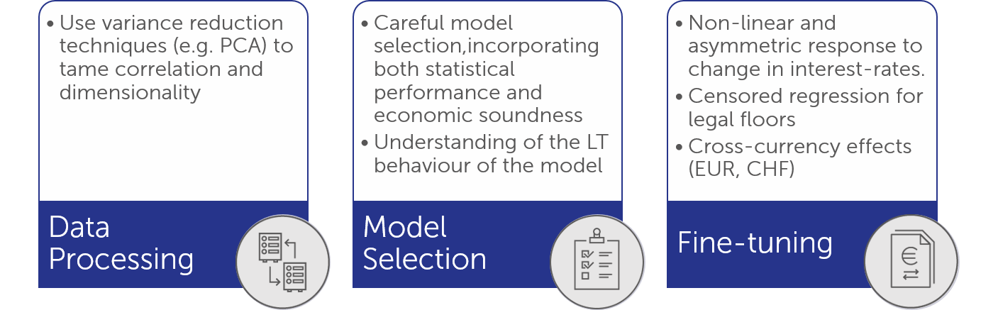
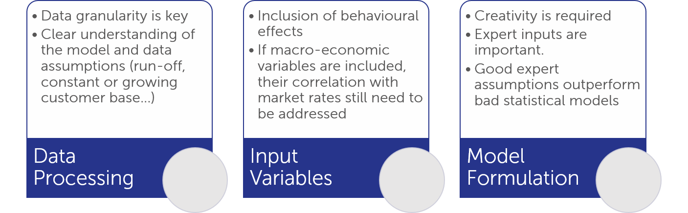
The models are therefore not only able to perform accurate projections on the short-term, but also on the long-term. Curiously enough, the best models were based on swap rates for overnight rates, and on government rates for time deposits. For overnight deposit, the quality of the fit is slightly deteriorated from 2013 onwards, but model performance may be improved by properly handling the legal floor of the deposit rate (using a censored regression), and by introducing an asymmetry in the adjustments of the rates (banks are usually faster to reflect decrease in rates to their customer than the opposite). Incorporating information from yield curve of other currencies may also be useful, especially if foreign-currency deposits are used e.g. as a protection against inflation. The key attention points are summarized in Figure 8.
Volume modelling is probably the most complicated part of NMD modelling, and the most demanding in term of data. Let us assume that \(B_t^k\) is the balance of account \(k\) at time \(t\) and that snapshots of balances of accounts are available at a given unit frequency. Then, the evolution of the volumes can be broken down in four components:
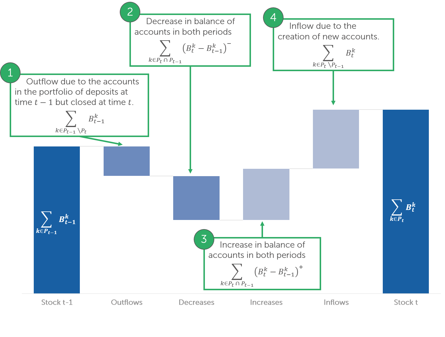
Each term can then be modelled using specific and tailored formulations. For instance, inflows are typically provided using assumptions from the budget plan. On the other side, outflows may be derived using hazard rate models, and increases and decreases using classical time series methods. In the process, it is still possible to separate the core balances which are likely to be unaffected by change in rates. It is also advised to perform the modelling at product level, since transactional and non-transactional accounts will have a very different behaviour. The set of explanatory variables may be extended to include customer information (e.g. age, behaviour), macro-economic factors such as the inflation, and even features of agent-like models (such as the difference in return between different investment opportunities). The models are nevertheless likely to differ significantly from one institution to the other, because the amount of deposits is largely driven by behavioural factors.
Finally, it should be noted that the distinction between the different components in the deposit flows depends on two hidden assumptions:
Different model formulations are also possible. For instance, using ECM has the advantage of introducing a target deposit level that each customer will try to achieve. This feature is interesting for transactional accounts and savings account, since clients tend to keep a fixed safety buffer on their overnight accounts and to invest the excess money in more lucrative financial instruments (e.g. stocks, bonds, funds, etc.). Otherwise, a seasonally adjusted ARIMA model may provide a more general framework.
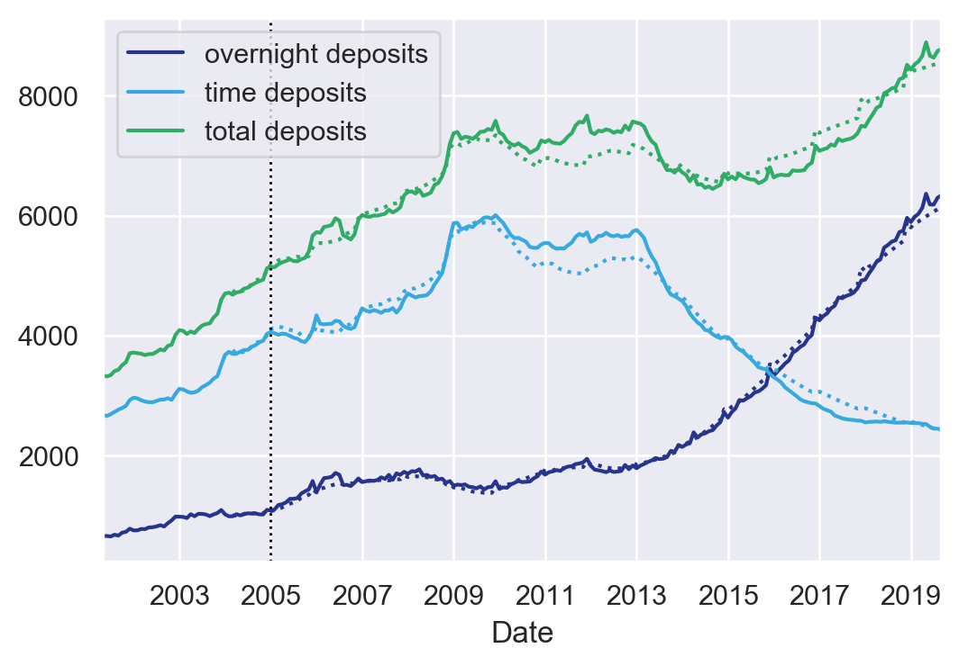
In order to illustrate the type of problems one can face in volume modelling, we designed a model for the total amount of overnight and time deposits in Hungary, retrieved from the statistical data warehouse of the MNB1. A key feature of these time series is the apparent outflow from time deposits to overnight deposits taking place from 2013 onwards. In order to capture it, the following explanatory variables were included in the model:
1. Hungarian Central Bank
A vector error correction model was retained, whose results are reported in Figure 10 (dotted lines are out of sample predictions starting from 2005 onwards). The model perfectly captures the increase in in time deposits in end 2008, and the flows between the different type of deposits from 2013 onwards.
In the case of the deposits of a single institution, the behavioural effects are likely to be more significant that what was observed in this example, which may require creative modelling. It is therefore important to have a proper business understanding of the portfolio and to use expert assumptions when necessary. The main attention points for volume modelling are therefore summarized in Figure 11.
In the current low-interest rate environment, the modelling of non-maturity deposits has attracted interests from Banks. These models are used for critical purposes in banks such as the management of the interest rate risk of the balance sheet, or in their earnings, as it is now also expected from supervisory authorities. Finally, they are also used to determine of a transfer price for deposits, in order to retribute the business lines in charge of collecting the deposits appropriately.
This blogpost has illustrated the key challenges faced in the modelling of non-maturity deposits, and Finalyse can be a key player in the enhancement of your non-maturity deposit framework modelling.
Finalyse InsuranceFinalyse offers specialized consulting for insurance and pension sectors, focusing on risk management, actuarial modeling, and regulatory compliance. Their services include Solvency II support, IFRS 17 implementation, and climate risk assessments, ensuring robust frameworks and regulatory alignment for institutions. |

Check out Finalyse Insurance services list that could help your business.
Get to know the people behind our services, feel free to ask them any questions.
Read Finalyse client cases regarding our insurance service offer.
Read Finalyse blog articles regarding our insurance service offer.
Designed to meet regulatory and strategic requirements of the Actuarial and Risk department
Designed to meet regulatory and strategic requirements of the Actuarial and Risk department.
Designed to provide cost-efficient and independent assurance to insurance and reinsurance undertakings
Finalyse BankingFinalyse leverages 35+ years of banking expertise to guide you through regulatory challenges with tailored risk solutions. |

Designed to help your Risk Management (Validation/AI Team) department in complying with EU AI Act regulatory requirements
A tool for banks to validate the implementation of RWA calculations and be better prepared for CRR3 in 2025
In 2027, FRTB will become the European norm for Pillar I market risk. Enhanced reporting requirements will also kick in at the start of the year. Are you on track?
Finalyse ValuationValuing complex products is both costly and demanding, requiring quality data, advanced models, and expert support. Finalyse Valuation Services are tailored to client needs, ensuring transparency and ongoing collaboration. Our experts analyse and reconcile counterparty prices to explain and document any differences. |

Helping clients to reconcile price disputes
Save time reviewing the reports instead of producing them yourself
Helping institutions to cope with reporting-related requirements
Be confident about your derivative values with holistic market data at hand
Finalyse PublicationsDiscover Finalyse writings, written for you by our experienced consultants, read whitepapers, our RegBrief and blog articles to stay ahead of the trends in the Banking, Insurance and Managed Services world |

Finalyse’s take on risk-mitigation techniques and the regulatory requirements that they address
A regularly updated catalogue of key financial policy changes, focusing on risk management, reporting, governance, accounting, and trading
Read Finalyse whitepapers and research materials on trending subjects
About FinalyseOur aim is to support our clients incorporating changes and innovations in valuation, risk and compliance. We share the ambition to contribute to a sustainable and resilient financial system. Facing these extraordinary challenges is what drives us every day. |

Finalyse CareersUnlock your potential with Finalyse: as risk management pioneers with over 35 years of experience, we provide advisory services and empower clients in making informed decisions. Our mission is to support them in adapting to changes and innovations, contributing to a sustainable and resilient financial system. |

Get to know our diverse and multicultural teams, committed to bring new ideas
We combine growing fintech expertise, ownership, and a passion for tailored solutions to make a real impact
Discover our three business lines and the expert teams delivering smart, reliable support