In this post, we present a comprehensive summary and commentary of (Halperin, 2020). We address one of the issues of the Black-Scholes model, which is the premise that a perfect hedge is possible, which is not true in the real world. One of the reasons behind this inefficacy is the assumption of continuous portfolio rebalancing. We present a discrete setup of the model and show how to solve it with reinforcement learning techniques.

In this post, we

1. Revisit the classical derivation of the BS equation via the delta-hedge argument.
2. Describe a discrete version of the BS model.
3. Provide a primer on Q-learning.
4. Show how to use it to solve the discrete BS model.

Particularly, we obtain a reinforcement learning algorithm that can solve the discrete BS model optimization problem. Its solution provides both an optimal hedge and an option price simultaneously. This is precisely the QLBS model introduced by Halperin.

Let B_t  be a risk-free bank deposit and S_t  be a stock value. We assume that there is a risk-free rate r and that S_t  follows the log-normal distribution with some fixed volatility σ  and drift μ , i.e.,

Our aim is to construct a hedge portfolio for this option. We denote the portfolio value at time t by Π_t . We assume that the portfolio consists only of stock shares and money and that it covers the payoff at the termination, i.e.,

where u_t  and x_t are the amounts of shares and money held in the portfolio at time t  according to the specified strategy. The crucial assumption we make is that the portfolio is self-financing, which means that the change in its value comes only from the change in the value of instruments held. Mathematically, this can be expressed as

cf. this post for an intuitive explanation of the formula. We want to determine how much money and stock to keep in the portfolio at each time to cover the option price. In our model, the option price V_t depends only on the current stock price and current moment in time, i.e., V_t=V(S_t,t). We therefore use Itô's lemma and obtain that

Equating the risky and riskless parts of equations (1) and (2) shows that a perfect hedge is possible for

This is the proclaimed delta-hedge strategy. The name comes from the fact that ∂V_t / ∂S  is precisely the delta of the option. Since V_T=H(S_T)=Π_T^BS  and since V_t  and Π_t^BS have the same dynamics under this strategy, we obtain that V_t=Π_t^BS  at each time, which means that we have a perfect hedge. The relation V_t=Π_t^BS  is therefore the renowned Black-Scholes equation,

We assume that we can only observe the world in between discrete time-step intervals Δt  (corresponding to the rebalancing frequency assumed by the trader). This results in the following bank account dynamics:

We again consider a self-financing hedge portfolio Π_t  with the terminal condition  Π_T= H(S_T).  Remember that the self-financing condition says that any change in the portfolio value comes from the change of the value of the instruments held. In our setting,    

This relation allows to express x_t  in terms of u_t, S_t+1, B_t/γ  and Π_t+1 , thus henceforth we will disregard x_t and associate the strategy (u_t,x_t) with (u_t)  only. Additionally, we have the following recursive relation:

From a trader’s perspective, for a given hedge strategy (u_t), the option ask price at time t, C_t, is the average hedge cost, V_t=E[Π_t | S_t], plus some risk premium. Mathematically speaking, this can be expressed in the following way:

While in the BS world, the risk premium is zero due to the existence of the perfect hedge, in the discrete world, the premium is proportional to the risk taken. Therefore, a natural choice of the optimal hedge strategy, when minimizing risk, is the one that minimizes the uncertainty at each step, i.e.,

Using only the recursive relation (3), the optimal solution can be found analytically to be

Assuming log-normal distribution of the underlying and taking the limit  Δt→0 retrieves the delta-hedge strategy described in the previous section, i.e.,

We have made a step towards generalizing the Black Scholes model. With our current setup, we can find the option ask price C_t and an optimal strategy using the standard backward algorithm (this requires assuming the underling dynamics and the risk premium formula). In the following sections, we introduce a reinforcement learning algorithm and then extend the above formulation even further to the form that can be solved with the use of the algorithm. As a result, we will obtain a method for calculating both hedge and price simultaneously without any underlying dynamics assumptions.

Let us take a small detour and talk about Q-learning which is a reinforcement learning (RL) algorithm.

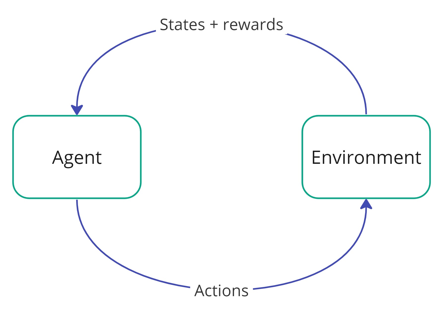
The basic setup of RL is that we have an agent and an environment. The agent observes a state of the environment, based on which they take an action, which results in a new state, based on which a new action is taken, etc. until some terminal condition occurs. Additionally, each state-action pair is associated with some reward returned by the environment, which tells how preferable being in the corresponding state and performing the action is.

The main goal of an RL algorithm is to learn a set of rules which tell the agent which action to take depending on the current state. Such set of rules is called a policy. Mathematically, a policy π is just a function that takes arguments in the state space and returns values in the action space, i.e., π(s)=a means that the agent should choose an action a, whenever in a state s. One can also consider random policies (with a random distribution over the action space) but here we restrict our attention to deterministic ones.

How to determine which action to take? As mentioned, moving with an action a from a state s to a state s', results in a reward, which we denote by R(s, a, s'). The total reward related to a policy π is the sum of the discounted future rewards, i.e.,

where S₀, S₁,…  are the consecutive state realizations, γ  is the discount factor and T  is the time horizon (can be infinite). Note that, as the environment can be random, states S_t are also random and so is G_t^π. An optimal policy π* is the one that maximizes all expected discounted future rewards, i.e.,

How to find π*? There are various approaches to that problem. One prominent example is the Q-learning algorithm, which we describe below.

A Q-function is a function that tells what the expected future reward is if the agent in a state s chooses an action a first and then follows a policy π. Mathematically,

The total reward for the optimal policy is equal to the immediate reward resulting in performing optimal action at the current state and then total reward coming from following the optimal policy, which is mathematically expressed as

Therefore

which is called Bellman’s optimality equation.

If we assume that our state process S is Markovian, then Q_t becomes independent of t. Q-learning algorithm is a value-iteration algorithm, which can then be described as follows:

1. Begin with random initial family (Q_t) and some initial state S_0. Fix learning rate α∈(0,1).
2. At time step t, pick a_t=argmax_a Q(S_t, a).
3. Apply action a_t, get to the next state S_t+1 and observe reward R(S_t,a_t,S_t+1).
4. Update Q-function:

1. Set t←t+1  and go to p. 2 until arriving at the termination state.
2. Repeat steps 2-5 with the newly-obtained family (Q_t)  and new state samples.

This procedure is guaranteed to converge given enough training data, and results in an optimal Q-function (more precisely, a family (Q_t) of Q-functions, if we have a time dependent case). This is a simple version of the algorithm, which has many alternative approaches that fix some of the issues (e.g., it can be accelerated if step 6. is performed batch-wise, or the convergence can be improved if in step 3. we choose a_t in ε-greedy fashion). For a more detailed view of the RL methods, we recommend this blog.

The optimal policy at time t can then be easily read from Q,

Above, we have silently assumed that the state-action space is finite (in which case given enough training data, the above procedure always converges). This assumption is crucial for the standard Q-learning algorithm and makes Q simply a table of values indexed by (state, action) pairs. There are multiple extensions (e.g., fitted Q-iteration, deep Q-learning), which allow getting rid of this assumption and use a functional approximation to the Q function, but pursuing this direction is beyond the scope of this blog post. Here, we just mention that those difficulties can indeed be overcome.

After the above recap, let us see the problem of the portfolio hedging in the discrete BS model via the lens of Q-learning notation.

In our setting, stock value space is the state space, and actions are associated with the amount of the stock kept in the hedge portfolio, while the policy tells us how much stock to keep, given its value: π(s_t)=u_t. Remember the option ask price formula C_t=E[Π_t+risk premium(t) | S_t] .

Let us try to define the total reward in the model. From the trader’s perspective, being able to hedge the position better (lower risk) results in a lower ask price. Therefore, a trader’s total reward is negatively proportional to the ask price. Ignoring the positive multiplicative factor, we can thus set:

We still need to define the risk premium, which is a component of C_t . (Halperin, 2020) gave the following definition in the spirit of Markovitz portfolio optimization theory:

where λ≥0  is the risk aversion parameter. The total reward is then given by

Note that we have not assumed anything about local rewards. We do not even know yet if the total reward can be decomposed into the sum of local rewards as was the case in the previous section. In fact, such decomposition is not required, as for our algorithm to work, we only need to have (some sort of) Bellman’s optimality equation, which we will obtain soon.

For now, we can show the formula for the Q-function. Remember that it is the expected total reward given that we are in a specified state, do a specified action and then follow a specified strategy. Therefore

Using only the recursive relation (3), tower rule and defining the one-step reward to be

(Halperin, 2020) proves the following Bellman’s optimality equation

Assuming that we are not policymakers (i.e., the stock value is independent of our actions), we can now use Bellman’s equation to easily solve analytically for the best policy

Note that the only difference between (4) and (5) lies in the last parameter EΔS_t/2γλ. This is consistent with the fact that in (4) we are only minimizing the risk, while in the total reward G_t^π, we also have a linear term -Π_t, which makes the resulting hedges different. In a sense, (5) is a generalization of (4), and (4) can be retrieved from (5) by setting λ= ∞ (i.e., pure risk minimization).

If we have access to transition probabilities (i.e., we make some strong model assumptions), then (5) is already good enough and can be solved by the dynamic programming techniques (in the spirit of American option valuation using Longstaff-Schwarz method).

However, the main observation is that we can go model-free already from Bellman’s optimality equation (BE). Thanks to the fact that we have formulated our problem in the language of RL, we can apply the Q-learning algorithm introduced previously directly to (BE). This has a huge advantage being that we do not need any model assumptions and can train the resulting QLBS algorithm using either synthetic or real data.

The additional advantage of learning the Q-function directly (via the Q-learning) is that having the Q-function, we can read from it both the option price and the optimal hedge strategy at the same time without any need for additional computation. We simply have

and

One technical difficulty that must be overcome in the Q-learner approach is that the state space is not discrete by default. This is either circumvent by discretizing the state space or by applying the beforementioned function expansion method of the Q-function (e.g., fitted Q-learning approach). We refer to (Halperin, 2020) for more details.

Let us summarize some main take-away points:

1. Among many issues, the BS model does not handle mis-hedging risk due to the continuous rebalancing assumption.
2. The discrete BS model removes this assumption and thus generalizes the BS model.
3. The discrete model can be solved numerically:
   1. Using dynamic programming if the transition probabilities are assumed.
   2. Using variants of the Q-learning algorithm under no model assumption (i.e., no underlying dynamics, such as log-normal distribution, is required to be known and we can train the model directly from the observed data).
4. The solution in QLBS yields the optimal hedge and the option values simultaneously as a part of the model.