In July 2025, the European Banking Authority (EBA) published the draft Guidelines on Credit Conversion Factor (CCF) estimation and application methodologies (hereafter, draft CCF GLs) for public consultation, which is scheduled to conclude on 29 October 2025. These draft CCF GLs represent a significant milestone in the history of CCF models, as they mark the first comprehensive formalization by the EBA of regulatory expectations and interpretations under the CRR framework. While the document is still in the draft form, it provides valuable insight into the regulatory vision of the future of the CCF models, enabling industry experts to assess potential impacts and prepare for the coming changes.
This blogpost is to analyze the implications of selected changes introduced in the draft CCF GLs. Specifically, it will assess the direction of the expected impact of these changes on existing CCF models and respective RWA (risk-weighted assets) impacts, and evaluate the operational and methodological adjustments likely required from banks’ modelling teams to align their current IRB (Internal Rating Based) models to the new regulatory environment.
The analysis provided focuses specifically on aspects most relevant to the model development process for retail portfolios.
Part 2 explores the CCF in default, analysing the approaches for incorporating incomplete recoveries into CCF models and the handling of post-default drawings, in particular details the allocation between CCF and LGD.
The CCF is one of the three parameters making up the A-IRB models. Its role is to calculate a bank's exposure to off-balance-sheet items. In essence, a CCF is a percentage used to estimate the portion of an undrawn credit commitment that a borrower is likely to draw down between the estimation date and the time of default (ToD).
As per Regulation (EU) 2024/1623 (known as CRR3), the CCF should be defined as:
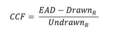
where  is the amount drawn at ToD,
  - amount drawn at the time of the estimation (reference date
  and
and  - undrawn limit at the time of the estimation.
As outlined earlier, Article 182(3) of CRR3 allows institutions to decide whether to include DaD in their CCF estimates, provided consistency with LGD is maintained. If this option is chosen, all DaD must be reflected in the realized CCFs.
Consistent with LGD practices, observed average CCF should be calculated only for facilities with a complete drawing process (terminated, fully repaid, written off, reclassified as non-defaulted, or those that reached the maximum recovery period). To derive the LRA CCF, this observed average CCF must however be adjusted for the most recent information on facilities with incomplete drawing processes.
According to the draft CCF GL, future unrealized drawings may be estimated through two approaches for non-retail exposures (simple approach, when modelling is disproportionate relative to having more reliable estimates, and modelling approach), while for retail exposures institutions deciding to include DaD in CCF must apply a modelling approach aligned with LGD methodology.
The draft CCF GLs clarify and operationalize the treatment of incomplete recoveries within the CCF risk parameter. This clarification builds on the existing requirements set out in CRR3 and on established in EBA/GL/2019/03 principle of exposure definition consistency between LGD and CCF.
To implement the modelling approach in accordance with potential regulatory requirement, the following steps should be taken at the model development stage:
The introduction of incomplete recoveries as part of the CCF in-default concept is expected to increase RWA compared to the current approach, where banks without in-default CCF models assigned a value of zero to defaulted exposures, assuming that no further changes in exposure are foreseen. However, this increase is expected to remain limited, as the proportion of defaulted exposures in the application portfolio is relatively small compared to banks’ overall portfolios. Furthermore, additional drawings after default are not expected to be common in the retail segment, as banks are generally expected to restrict such drawings through their internal lending standards.
Additional drawings after default (DaD) are the funds that a borrower withdraws from an available credit line or facility after a formal default event has occurred. For example, in case of a credit card exposure, the borrower might have defaulted on a consumer loan but still has the capacity to withdraw money on their credit card and, hence, has additional post-default drawings.
Article 182(1)(c) of the CRR3 stipulates that CCF estimates must include additional DaD. However, Article 182(3) introduces an amendment for retail exposures, allowing institutions to allocate post-default drawings either to the CCF or to the LGD estimates.
In the presence of post-default drawings, the CCF formula can be rewritten as:
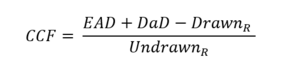
where DaD – are the drawings after default. Traditionally, this DaD is measured by adding all additional drawings to the EAD after discounting:
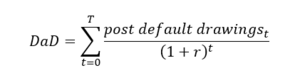
In a “going concern” obligor does large post default drawings, such formula can lead to very high additional drawn amounts and thus high observed CCFs and low LGDs. This effect will be compounded in case of very granular data on drawings and recoveries, i.e. when a bank observes all the post default drawings and reimbursements and not only the monthly difference in the balance amount.
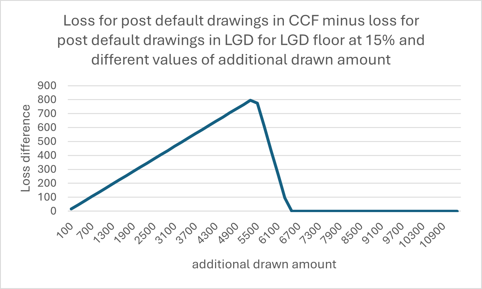
At the level of the measured loss, these two effects will cancel out. However, in case a model does not perform perfectly (which is expected), the processing of additional drawings can bias the RWA results. Such potential biases are amplified by the floors for the parameters’ quantification: for some retail products we have difference between the floor for LGDs and for CCFs, while the integration of the post default drawings can be incorporated in either parameter at the discretion of the modeler.
This difference in floor value can lead to an “arbitrage” between CCF and LGD definitions, resulting in a difference in RWA. To illustrate this point, let’s consider the following simple illustrative example of a small business owner classified as retail and having a small business line of credit. After the loan has defaulted, the line of credit remains classified as in default, although the bank does not prevent the obligor from continuing to draw additional funds.
Let’s suppose that 12 months before the default the drawn amount is €1K and the undrawn amount €4K. The EAD is €3K, the additional drawn amount (calculated as the sum of the discounted post default drawings) is €4K and recoveries (including the fees capitalized after default) amount to €8K. We get the following parameters for the two possible methodologies:
| CCF | LGD | Expected Loss for LGD floor of 0% | Expected Loss for LGD floor of 15% |
Post default drawings in CCF | 150% | -14.29% | 0 | 1050 |
Post default drawings in LGD | 50% | -33.33% | 0 | 450 |
By applying the 15% LGD floor for other retail exposures secured by other physical collateral, we get the different levels of expected losses when including the post default drawings into the LGD or into the CCF. Such floor is in practice applied at the LGD estimate level (i.e., calibration level), but here in our simplifying example there is only one exposure so we apply it at the exposure level. Continuing with our illustrative example, we can see that changing the post-default drawing amount will change the difference in measured loss between including it into the CCF and into the LGD. This loss difference relation is non-linear and becomes 0 as the LGD without including the post default drawings exceed the 15% threshold:
To avoid very high realized CCFs and very low realized LGDs, the draft CCF Guidelines propose to calcule the additional drawings as the difference between the exposure at default and the highest discounted drawn amount observed during the default period.
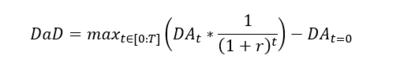
There are two major differences in this new formula. The first one is that the full drawn amount is discounted at the considered date instead of discounting each drawing at the date of its occurrence. The second primary difference is that the formula implicitly accounts for recoveries as the total drawn amount is affected by both drawings and repayments.
This new formula introduces a discrepancy compared to the existing methodology for incorporating additional drawings (for retail exposures) into the LGD, which is currently done as a sum of discounted cash flows. This inconsistency may lead to 'cherry-picking', i.e., selecting the calculation method that results in the lowest recognized losses.
This new definition of the additional drawn amount has the potential to drastically change the measured CCFs when the post-default drawings are an important component of the CCF. To illustrate this point, we will take a simple example.
Let’s suppose again that 12 months before the default the drawn amount is €1K and the undrawn amount €4K. The amount drawn at default is €3K, the discount rate 5% and the post default drawings (positive amounts) and recoveries (negative amounts) are the following stream of cash flows:
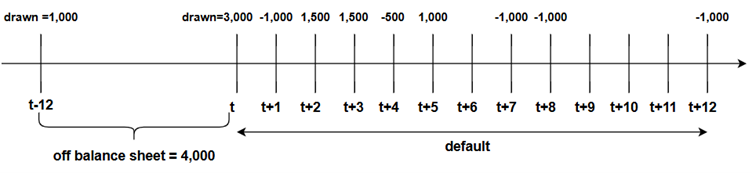
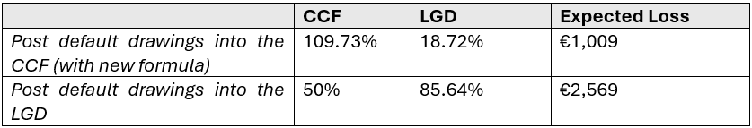
With the former formula (discounted sum of post default drawings), the additional drawn amount is €3,945.5. With the new formula, it becomes €2,389.3. We get the following parameters for the two formulae:
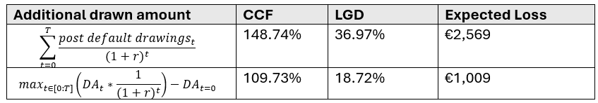
The new additional drawn amount formula, by reducing the value of the amount added to the drawn amount, decreases the recorded loss. For retail exposures, this creates an opportunity to select the lowest recorded loss by choosing between incorporating the post default drawings into the CCF or into the LGD:
Under the new regulation, additional drawings and recoveries are no longer fully reflected in the CCF, as the modelling now relies on the maximum drawn amount. As a result, the treatment of post-default drawings leads to different expected loss outcomes depending on the LGD’s position relative to its regulatory floor (e.g. 15% for revolving retail exposures secured by commercial immovable property).
As shown above, when the LGD exceeds its floor, allocating post-default drawings to the CCF produces lower expected losses than including them in the LGD. Conversely, when the LGD falls below its regulatory floor, it becomes more appropriate to include the post-default drawings in the LGD, consistent with the effect previously observed under the current definition of the additional drawn amount.
The new EBA formula changes the treatment of additional drawn amounts considerably, often resulting in a significant reduction depending on the timing of post-default drawings and recoveries. Consequently, it is expected to decrease the RWA for portfolios with substantial post-default drawings and will necessitate major updates to the CCF models currently used by banks. Furthermore, including post-default drawings within the LGD may be more beneficial, as LGD floors limit the potential reduction in capital if these drawings are accounted for in the CCF.
The draft CCF GLs explicitly set out methods for assigning CCF estimates to defaulted facilities when DaD are included in the calculation. For retail exposures, a modelling approach should be applied when estimating CCF in-default, while for non-retail portfolios an additional simplified approach is available.
The draft CCF GLs require that, consistent with the LGD framework for defaulted exposures, institutions implement a modelling approach where reference dates (potentially multiple) are determined based on observed post-default drawing patterns. For CCF in-default, the use of a fixed 12-month horizon is not permissible.
Institutions must also define a maximum drawing period, representing the time in default after which no further drawings are assumed possible. This period is expected to be aligned with the MRP (maximum recovery period) applied for LGD.
Consider an illustrative example with three facilities:
All three facilities exhibit additional DaD, as shown in Figure 2.
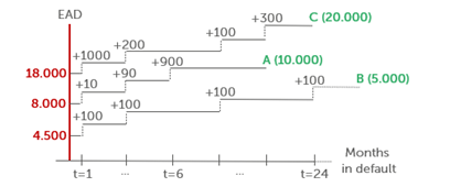
Figure 2: Illustrative example of drawings after default
Assume that based on the institution’s internal analysis of contractual practices defining DaD in the retail segment, it was observed that the drawing behavior changes materially after 6 months in default. Consequently, reference dates at 1 month and 6 months are defined for the purpose of CCF-in-default estimation, in line with the regulatory requirement to select reference dates based on observed post-default drawing patterns. Additionally, we assume that at portfolio level, no drawings or recoveries occur beyond 24 months in default. The institution therefore sets the maximum drawing/recovery period (MRP) at 24 months, aligned with both the EBA GLs and the maximum recovery period as defined in the LGD model.
The LRA CCF in-default will be calculated for each of the selected reference dates separately (LRA CC1, LRA CCF6 and LRA CCF24) and then applied to the facilities that are in default at least as long as the selected reference date (Table 3):
Facility | Time in default | Applied LRA |
W | 1 month |
|
X | 3 months |
|
Y | 8 months |
|
Z | 25 months |
|
Table 3: Example of application of the LRA CCFs by reference date
For each of the reference dates (Rk), the respective LRA CCF in-default is calculated as simple default-weighted average as follows:
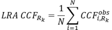
where  is the number of facilities that are in default at time
  is realized CCF of facility
  at time
  that is computed in accordance with the defined draft CCF GLs formula for CCF DaD as below:
where  are additional drawings on facility between the current reference date
  and T which corresponds to the end of default. The respective observed CCFs calculated on the defined example are shown in Table 4 (interest rate of 3% is considered when discounting the cashflows).
ID | Ref date | AD | CCF |
A | 1 | 879.83 | 44.21% |
A | 6 | 0.00 | 0.00% |
B | 1 | 88.44 | 22.11% |
B | 6 | 29.58 | 9.86% |
B | 24 | 0.00 | 0.00% |
C | 1 | 152.76 | 15.28% |
C | 6 | 0.00 | 0.00% |
C | 24 | 0.00 | 0.00% |
Table 4: Computation of the realized CCFs at reference date for the illustrative example
Having calculated the average realized CCF for each of the reference dates, the final LRA CCF in-default are shown in Table 5.
|
|
|
27.20% | 3.29% | 0.00% |
Table 5: Final calibrated CCF values by reference date
It should be noted that this illustrative example does not take into consideration incomplete recoveries. In case there are incomplete recoveries in the portfolio, the future drawings should be estimated for those facilities first and then the LRA CCF is computed based on the closed, reached MRP and adjusted open defaults.
The RWA impact of introducing CCF in-default concept into the model design is highly dependent on the institution’s existing post-default processes and modelling assumptions. Where the current framework assumes no DaD, the application of a positive CCF in-default will increase the EAD of defaulted facilities and, consequently, RWA. Conversely, if the current approach already accounts for DaD conservatively, replacing these assumptions with calibrated CCF in-default estimates, typically lower, may reduce RWA. Finally, in portfolios with contractual or operational practices of blocking credit limits at default, thereby preventing further drawings, the estimated CCF in-default will be close to zero, resulting in a negligible RWA impact.
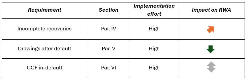
The table below summarizes the key focus areas of the draft CCF GLs outlined above and their expected impact on RWA (graphically in the respective column below). The requirements with “high” (red arrows) RWA impact are expected to cause the most noticeable increase in the RWA values. The implementation of the “medium” impact points (orange arrows) is expected to result in limited RWA increase. The remaining requirements are not associated with a predetermined increase or decrease in RWA, as their impact may vary depending on the characteristics of each individual portfolio.
In addition, the summary table provides an indicative assessment of the implementation effort required to adapt the existing models in the European banks (based on common market practices) to the draft requirements, should they come into force in the current form. In this context, low effort refers to adjustments such as sample filtering or model recalibration; medium effort corresponds to changes in risk differentiation or the reconstruction of risk driver functions; and high effort involves fundamental changes to model design and a full redevelopment.
Finalyse InsuranceFinalyse offers specialized consulting for insurance and pension sectors, focusing on risk management, actuarial modeling, and regulatory compliance. Their services include Solvency II support, IFRS 17 implementation, and climate risk assessments, ensuring robust frameworks and regulatory alignment for institutions. |

Check out Finalyse Insurance services list that could help your business.
Get to know the people behind our services, feel free to ask them any questions.
Read Finalyse client cases regarding our insurance service offer.
Read Finalyse blog articles regarding our insurance service offer.
Designed to meet regulatory and strategic requirements of the Actuarial and Risk department
Designed to meet regulatory and strategic requirements of the Actuarial and Risk department.
Designed to provide cost-efficient and independent assurance to insurance and reinsurance undertakings
Finalyse BankingFinalyse leverages 35+ years of banking expertise to guide you through regulatory challenges with tailored risk solutions. |

Designed to help your Risk Management (Validation/AI Team) department in complying with EU AI Act regulatory requirements
A tool for banks to validate the implementation of RWA calculations and be better prepared for CRR3 in 2025
In 2027, FRTB will become the European norm for Pillar I market risk. Enhanced reporting requirements will also kick in at the start of the year. Are you on track?
Finalyse ValuationValuing complex products is both costly and demanding, requiring quality data, advanced models, and expert support. Finalyse Valuation Services are tailored to client needs, ensuring transparency and ongoing collaboration. Our experts analyse and reconcile counterparty prices to explain and document any differences. |

Helping clients to reconcile price disputes
Save time reviewing the reports instead of producing them yourself
Helping institutions to cope with reporting-related requirements
Be confident about your derivative values with holistic market data at hand
Finalyse PublicationsDiscover Finalyse writings, written for you by our experienced consultants, read whitepapers, our RegBrief and blog articles to stay ahead of the trends in the Banking, Insurance and Managed Services world |

Finalyse’s take on risk-mitigation techniques and the regulatory requirements that they address
A regularly updated catalogue of key financial policy changes, focusing on risk management, reporting, governance, accounting, and trading
Read Finalyse whitepapers and research materials on trending subjects
About FinalyseOur aim is to support our clients incorporating changes and innovations in valuation, risk and compliance. We share the ambition to contribute to a sustainable and resilient financial system. Facing these extraordinary challenges is what drives us every day. |

Finalyse CareersUnlock your potential with Finalyse: as risk management pioneers with over 35 years of experience, we provide advisory services and empower clients in making informed decisions. Our mission is to support them in adapting to changes and innovations, contributing to a sustainable and resilient financial system. |

Get to know our diverse and multicultural teams, committed to bring new ideas
We combine growing fintech expertise, ownership, and a passion for tailored solutions to make a real impact
Discover our three business lines and the expert teams delivering smart, reliable support