In July 2025, the European Banking Authority (EBA) published the draft Guidelines on Credit Conversion Factor (CCF) estimation and application methodologies (hereafter, draft CCF GLs) for public consultation, which is scheduled to conclude on 29 October 2025. These draft CCF GLs represent a significant milestone in the history of CCF models, as they mark the first comprehensive formalization by the EBA of regulatory expectations and interpretations under the CRR framework. While the document is still in the draft form, it provides valuable insight into the regulatory vision of the future of the CCF models, enabling industry experts to assess potential impacts and prepare for the coming changes.
This blogpost is to analyze the implications of selected changes introduced in the draft CCF GLs. Specifically, it will assess the direction of the expected impact of these changes on existing CCF models and respective RWA (risk-weighted assets) impacts, and evaluate the operational and methodological adjustments likely required from banks’ modelling teams to align their current IRB (Internal Rating Based) models to the new regulatory environment.
The analysis provided focuses specifically on aspects most relevant to the model development process for retail portfolios.
Part 1 provides an overview of the proposed amendments to the calculation of the LRA CCF, focusing on the fixed 12-month horizon and the use of equal weights in the LRA framework. It also discusses the clarified definition of the Region of Instability (RoI) and its implementation.
The CCF is one of the three parameters making up the A-IRB models. Its role is to calculate a bank's exposure to off-balance-sheet items. In essence, a CCF is a percentage used to estimate the portion of an undrawn credit commitment that a borrower is likely to draw down between the estimation date and the time of default (ToD).
As per Regulation (EU) 2024/1623 (known as CRR3), the CCF should be defined as:
$$CCF = \begin{array}{c} EAD - Drawn_{R} \\ \hline Undrawn_{R} \end{array}$$
where  is the amount drawn at ToD,
  - amount drawn at the time of the estimation (reference date
  and
and  - undrawn limit at the time of the estimation.
The 12-month fixed horizon requirement establishes that the reference date for CCF estimation must be selected as 12 months prior to default date. This requirement was introduced under CRR3 Art. 182(g), para. 3 and came into effect from 1st of January 2025. It was further detailed in the draft CCF GLs.
The requirement implies that risk differentiation and quantification must be based exclusively on the snapshots corresponding to 12 months prior to default. In case of “fast defaults” (defaults occurring within 12 months of origination), a retracted reference date must be applied as these exposures cannot be omitted [CRR3, Art. 182(1)(a)]. In most cases, the retracted reference date corresponds to the earliest date at which both the exposure amount and limit are reliably observed, typically the origination date. When including “fast default” into the model, additional adjustments must be made to prevent bias in the CCF estimates (appropriate adjustment or a MoC).
In general, the undrawn amount is larger at 12 months before default than at dates closer to default, providing the borrower with more time for drawings until the default. Consequently, observed CCFs tend to be higher when measured from the 12-month reference date and generally decrease as the reference date approaches the ToD. Given that, the approaches commonly used by European banks, such as the cohort and random selection methods, may underestimate LRA CCFs relative to the 12-month fixed horizon methodology. It should be noted that bank-specific processes, such as borrower-requested changes to credit limits, may influence this pattern and should be considered when assessing the impact on RWA.
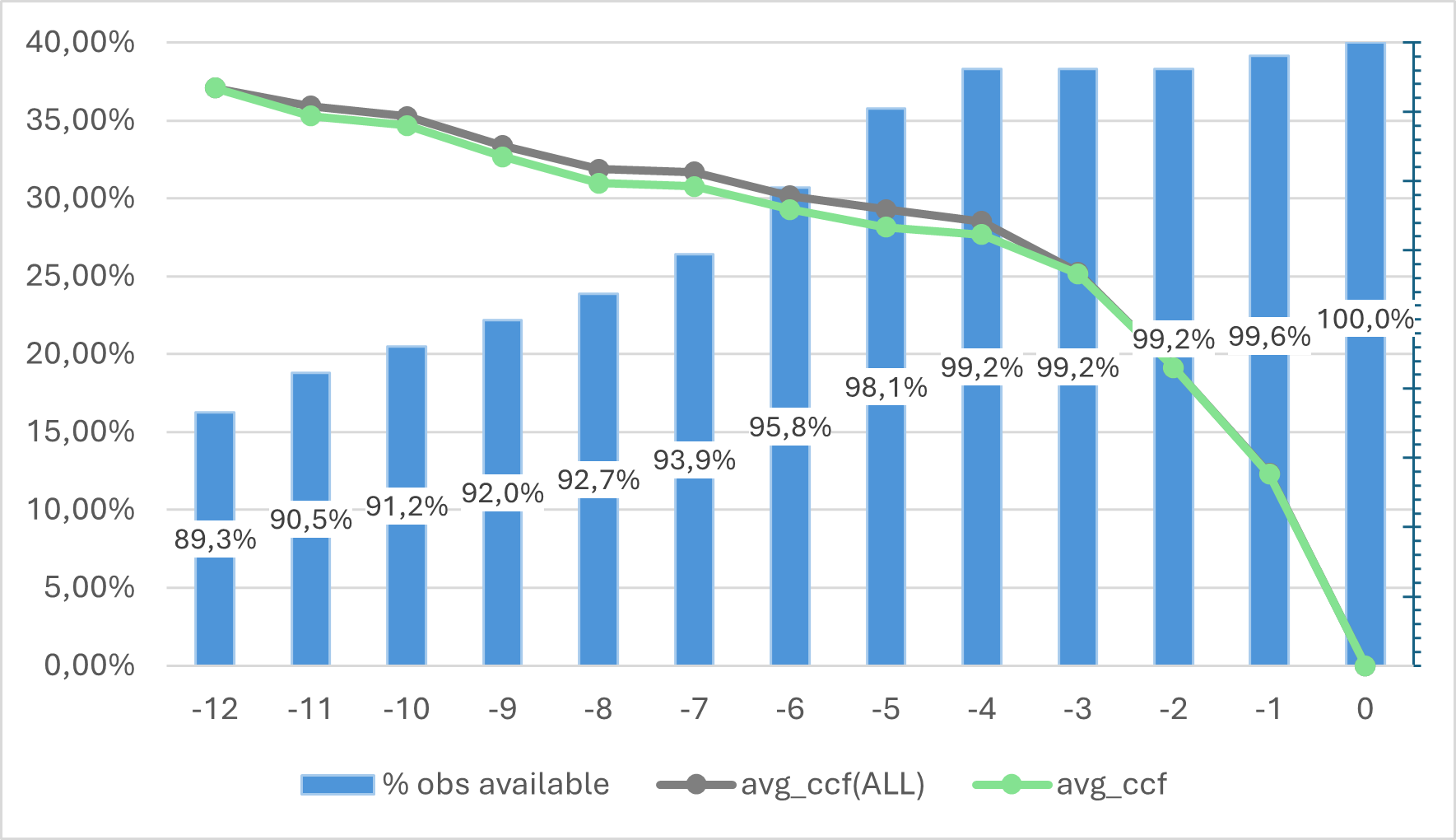
Figure 1: Observed average CCF by time to default and share of defaults observable in each sample month t
The illustrative example in Figure 1 demonstrates that the average observed CCF consistently decreases when moving from 12 months prior toward ToD. To assess the impact of the 12-month fixed-horizon requirement, this LRA CCF value is compared with the LRA CCFs obtained using two commonly applied methodologies: the random selection approach and the cohort approach. A summary of these results is presented in Table 1.
Scenario | LRA CCF |
Random selection | 29.00% |
Cohort approach | 28.94% |
Fixed 12 months, w “fast defaults” | 39.49% |
Fixed 12 months, w/o “fast defaults” | 37.08% |
Table 1: 12-month fixed horizon impact on LRA CCF
This evidence suggests that applying a fixed 12-month horizon, rather than relying on a randomly selected reference date or cohort approach, leads to systematically higher CCF estimates. For the portfolio under consideration, the shift in the LRA computation approach results in an increase of approximately 10% in the LRA CCF. Consequently, the use of the fixed horizon approach is expected to increase the RWAs as well.
Additionally, the example shows that including “fast defaults” in the LRA CCF calculation for the selected retail portfolio does not compromise the conservatism of the resulting CCF estimates.
As a result, banks whose CCF models do not currently rely on 12-month fixed horizon will need to review their frameworks. This will require not only methodological adjustments but also a careful quantification of the potential increase in RWA, to ensure that the models remain fully compliant once the proposed CCF GLs enter into force.
The draft CCF GL provide a clearer definition and specific guidance for the treatment of fully, and nearly fully, drawn facilities (Region of Instability, hereafter, RoI), where the low undrawn amounts in the CCF denominator can lead to unstable or extreme CCF values.
The previously existing expectation to isolate the facilities with unstable CCF within the region of instability (EBA/GL/2017/16), already established in the context of PD and LGD modelling, has now been explicitly formalized for CCF models. In addition, the draft CCF GLs introduced several new requirements specific to the treatment of RoI exposures in CCF estimation.
RoI segment CCF computation. For facilities within the RoI, realized CCFs must be computed using the Limit Factor (LF) approach, defined as the ratio of the drawn amount at default to the total limit at the reference date. In application, the EAD is approximated by the application of LF to the observed credit limit amount.
$$LF_{t} = \begin{array}{c} EAD \\ \hline Limit_{t} \end{array}$$
The draft CCF GL reiterate that institutions are not permitted to exclude, cap, or truncate extreme or unstable CCF observations. In line with the principles set out in CRR3 (Art. 182(1)(b)), such observations must be incorporated into model calibration, with appropriate segmentation applied where relevant to ensure robust and reliable CCF estimates.
Consider an example of facility A which has a utilization rate of 99% and can be considered almost fully drawn and hence, corresponding to the RoI region (see Table 2).
ID | DrawnR | LimitR | UndrawnR | EAD | UsageR | CCF | LF |
A | 99 | 100 | 1 | 99.9 | 99.00% | 90.00% | 99.90% |
Table 2: RoI example, neutral impact
For this facility, computation of realized CCF in accordance with the common framework results in:
$$CCF_{A} = \begin{array}{c} EAD_{A} - Drawn_{R,A} \\ \hline Undrawn_{R,A} \end{array} = \begin{array}{c} 99.9 - 99 \\ \hline 1 \end{array} = 90\%$$
Following the framework of LF computation, the result for facility A would be:
$$LF_{A} = \begin{array}{c} 99.9 \\ \hline 100 \end{array} = 99.9\%$$
In the application portfolio, consider a facility B with LimitApp=100, DrawnApp=99, which is segmented into RoI as an almost fully drawn facility. The respective EAD computed under CCF and LF approach are identical for this example:
$$EAD_{B}^{CCF} = CCF \times Undrawn_{B} + Drawn_{B} = 0.9 \times 1 + 99 = 99.9$$
$$EAD_{B}^{LF} = LF \times Limit_{B} = 99.9 \times 100 = 99.9$$
For the individual facility B in the application portfolio, the EAD impact of switching from CCF to LF parameters is neutral. However, at the portfolio level, the effect can differ. Since fully drawn facilities are generally associated with higher realized CCFs, their exclusion from the CCF region may lead to a decrease in the LRA and, consequently, a reduction in EAD. This effect arises from the relatively large exposure within the CCF region in the application portfolio.
Nevertheless, the impact is not unidirectional. Almost fully drawn facilities are often very unstable: small relative changes in exposure between the reference date and the default date can result in substantial variations in observed CCFs.
Consider, for example, the three facilities shown in Table 3. For these facilities, exposure changes of only a few cents between the reference and default dates lead to significant fluctuations in observed CCFs. If such facilities are retained within the CCF region, the LRA CCF may become severely unstable and in this example biased downward due to the presence of low or even negative realized CCFs. In contrast, realized LF values remain relatively stable after small changes in exposure
ID |
|
|
|
|
|
|
|
| 99.9 | 100 | 0.1 | 99 | 99.90% | -900.00% | 99.00% |
| 99.9 | 100 | 0.1 | 99.91 | 99.90% | 10.00% | 99.91% |
| 99.9 | 100 | 0.1 | 99.8 | 99.90% | -100.00% | 99.80% |
Table 3: RoI example, positive impact.
In conclusion, the direction of the RWA impact stemming from the introduction of the LF factor as a parameter for estimating EAD for nearly or fully drawn facilities depends on the specific structure of the portfolio under analysis. However, in all cases, accurate identification of RoI facilities remains critical to maintaining stable and reliable estimates. From a technical standpoint, defining the rules to correctly isolate RoI facilities may entail substantial adjustments to the model’s specification and implementation.
The requirement establishes the methodology for aggregation of the individual realized CCFs to the calibrated LRA CCF value. In particular, the weighting of each individual contribution when calibrating to the LRA CCF.
Under the draft CCF GLs, the LRA CCF is computed as the arithmetic average of realized CCFs over the full historical observation period, weighted by the number of defaults. Unlike earlier guidelines, unequal weighting of historical periods or annual averaging should not be applied, ensuring that each default contributes proportionally to the LRA CCF estimate. Additionally, it is clarified in the draft CCF GLs, that the length of the calibration sample should be the same as that of the risk quantification sample.
For portfolios with concentrated default periods, the removal of annual averaging can either raise or lower the LRA CCF. The impact depends on the relationship between default frequency and realized CCFs. If years with higher number of defaulted exposures coincide with higher average CCFs, the LRA CCF will increase, if not, the effect may be neutral or negative.
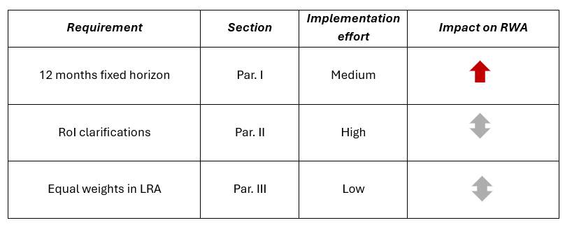
The table below summarizes the key focus areas of the draft CCF GLs outlined above and their expected impact on RWA (graphically in the respective column below). The requirements with “high” (red arrows) RWA impact are expected to cause the most noticeable increase in the RWA values. The implementation of the “medium” impact points (orange arrows) is expected to result in limited RWA increase. The remaining requirements are not associated with a predetermined increase or decrease in RWA, as their impact may vary depending on the characteristics of each individual portfolio.
In addition, the summary table provides an indicative assessment of the implementation effort required to adapt the existing models in the European banks (based on common market practices) to the draft requirements, should they come into force in the current form. In this context, low effort refers to adjustments such as sample filtering or model recalibration; medium effort corresponds to changes in risk differentiation or the reconstruction of risk driver functions; and high effort involves fundamental changes to model design and a full redevelopment.
Finalyse InsuranceFinalyse offers specialized consulting for insurance and pension sectors, focusing on risk management, actuarial modeling, and regulatory compliance. Their services include Solvency II support, IFRS 17 implementation, and climate risk assessments, ensuring robust frameworks and regulatory alignment for institutions. |

Check out Finalyse Insurance services list that could help your business.
Get to know the people behind our services, feel free to ask them any questions.
Read Finalyse client cases regarding our insurance service offer.
Read Finalyse blog articles regarding our insurance service offer.
Designed to meet regulatory and strategic requirements of the Actuarial and Risk department
Designed to meet regulatory and strategic requirements of the Actuarial and Risk department.
Designed to provide cost-efficient and independent assurance to insurance and reinsurance undertakings
Finalyse BankingFinalyse leverages 35+ years of banking expertise to guide you through regulatory challenges with tailored risk solutions. |

Designed to help your Risk Management (Validation/AI Team) department in complying with EU AI Act regulatory requirements
A tool for banks to validate the implementation of RWA calculations and be better prepared for CRR3 in 2025
In 2027, FRTB will become the European norm for Pillar I market risk. Enhanced reporting requirements will also kick in at the start of the year. Are you on track?
Finalyse ValuationValuing complex products is both costly and demanding, requiring quality data, advanced models, and expert support. Finalyse Valuation Services are tailored to client needs, ensuring transparency and ongoing collaboration. Our experts analyse and reconcile counterparty prices to explain and document any differences. |

Helping clients to reconcile price disputes
Save time reviewing the reports instead of producing them yourself
Helping institutions to cope with reporting-related requirements
Be confident about your derivative values with holistic market data at hand
Finalyse PublicationsDiscover Finalyse writings, written for you by our experienced consultants, read whitepapers, our RegBrief and blog articles to stay ahead of the trends in the Banking, Insurance and Managed Services world |

Finalyse’s take on risk-mitigation techniques and the regulatory requirements that they address
A regularly updated catalogue of key financial policy changes, focusing on risk management, reporting, governance, accounting, and trading
Read Finalyse whitepapers and research materials on trending subjects
About FinalyseOur aim is to support our clients incorporating changes and innovations in valuation, risk and compliance. We share the ambition to contribute to a sustainable and resilient financial system. Facing these extraordinary challenges is what drives us every day. |

Finalyse CareersUnlock your potential with Finalyse: as risk management pioneers with over 35 years of experience, we provide advisory services and empower clients in making informed decisions. Our mission is to support them in adapting to changes and innovations, contributing to a sustainable and resilient financial system. |

Get to know our diverse and multicultural teams, committed to bring new ideas
We combine growing fintech expertise, ownership, and a passion for tailored solutions to make a real impact
Discover our three business lines and the expert teams delivering smart, reliable support