

The highest possible predictive power of your models
How confident are you that your risk models show what you need to see? Would your regulator agree?
Model Validation: are you sure your internal risk parameter estimates are adequate, robust and reliable?
Control your model risk with the right tool to develop and validate models, bridge the talent gap and reduce implementation risks
Written by Long Le Hai, Consultant
The IFRS9 is a comprehensive replacement of IAS39 and requires major updates to calculate the provision for credit losses. The biggest change is credit impairment in expected credit loss (ECL) calculation which was updated regarding the consideration of forward-looking information.
Forward-looking information is a distinctive feature of an IFRS9 ECL model. Institutions are expected to update the macroeconomic forecasts to reflect the current and future state of the economy. Therefore, it is critical to incorporate macroeconomic factors to capture credit losses.
The estimated probability of default (PD) should include forward-looking information, whilst estimation of Lifetime PD should include macroeconomic factors. Many macroeconomic factors can be used as inputs for forecasting Forward-Looking Information PD for different economic scenarios.
Example of Macroeconomic Factors | |
Economic Output | Gross Domestic Product (GDP) |
Gross National Product (GNP) | |
Inflation | Consumer Price Index (CPI) |
Producer Price Index (PPI) | |
Deflators | |
Real Estate | House Price Index (HPI) |
Labour Markets | Employment |
Unemployment Rate | |
Interest Rate | ECB rate |
10-year government bond yields | |
Government Output | Budget Deficit |
Public Debt | |
Foreign Sector | Exchange Rates |
Current Account | |
Incorporating economically stressed states of the economy impacts IFRS 9 PD the most. Macroeconomic PD is also known as Point-in-Time (PIT) PD. PIT PD model has macroeconomic factors as independent variables, and the dependent variable is the 12-month Observed Default Rate (ODR).
The 12-month ODR will be predicted based on multiple macroeconomic factors by solving a multivariate time-series problem. This article outlines different methods to predict 12-month ODR; it will cover data collection, data transformation, feature engineering and variable selection. The characteristics, functionalities as well as strength and weaknesses of each algorithm will be discussed. Finally, this article will conclude with some closing remarks to determine the final model and the fit of these algorithms to predict the 12-month ODR of Point-in-Time PD.
Data is usually not ready to use and must be prepared first. Time-series macroeconomic data is collected as independent variables, and 12-month ODR as a target variable. Time-series is a sequence of data points collected over a time interval. There are some potential macroeconomic factors which can be collected for modelling purposes.
Generally, the longer the historical data, the more powerful the learning algorithms are. The time frame used for modelling should cover at least several, for example, 5 years. The modelling dataset should have macroeconomic factors (MF) and 12-month ODR for each time point in the selected frame. The sample dataset may have the following variables (with dummy data):
Period | GDP | HPI | CPI | GNP | Inflation | 12m ODR |
Jan-21 | 521 | 121 | 116 | 650 | 9.1 | 6% |
Feb-21 | 532 | 123 | 120 | 652 | 8.8 | 5% |
Mar-21 | 535 | 125 | 121 | 655 | 8.6 | 5% |
Apr-21 | 540 | 125 | 123 | 657 | 8.1 | 4% |
There are 2 main approaches: traditional multivariate time series and supervised machine learning. It is beneficial to apply data transformation and feature engineering to raw time-series MF data. With the transformation, the dataset is tabular and labelled to map inputs (MF) with associated outputs (ODR) so that machine learning algorithms can solve multivariate time-series problems. From this point onward, 12-month ODR will be called PIT PD for simplicity.
The purpose of feature engineering is to create more meaningful and explainable variables from existing variables. To improve the predictive power, it is important to engineer the features intuitively and effectively.
The features should be normalized or standardized to improve the interpretability and functionality of learning algorithms. This step applies a common scale to all the features and prevents distorting the differences in the ranges.
Lagging is the simplest and most popular way of transforming existing variables into new ones. It is possible to create various lag features for a variable. Depending on expert knowledge, it can be useful to include lag features from last 6 months, 1 years, 2 years, etc.
Other feature engineering techniques include Rolling Mean, Difference, and Quotient. These techniques will inevitably produce missing values in the first few periods of the dataset. If the number of observations is sufficient, the first few rows that have missing values can be removed to have a complete dataset.
More advanced feature engineering techniques include:
Example of Feature Engineering of EU Inflation Rate with Lag2, Difference2, Quotient3, RollingMean2 using Dplyr package in R:
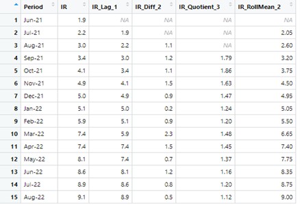
Feature engineering allows one variable to be used in different contexts, which can be more appropriate in the modelling process. It creates a larger set of potentially useful variables. For instance, Rolling_Mean(2) of the Inflation Rate captures the short-term trend. However, the final model cannot include all features because of model overfitting and multicollinearity; the variable Selection step is necessary.
Variable Selection aims to select the ‘best’ subset of predictors to include in the model. Both qualitative (expert knowledge) and quantitative (statistical methods) processes can be applied to Variable Selection. Statistical variable selection is a critical step of supervised learning regression. Multiple methods can be implemented in this process; for example, Ridge Regression, which can be used for OLS, and VarImp (Variable Importance), which can be used for XGBoost.
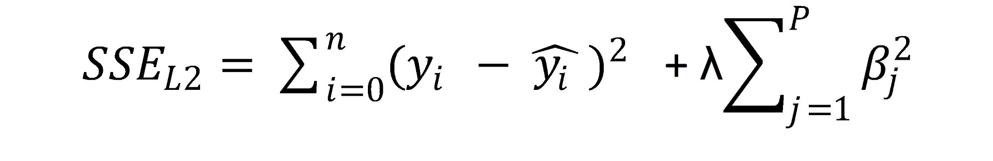
The consequence of introducing this error term is that only the most significant variables are assigned a significantly non-zero coefficient to minimise the overall error term. As a result, only these variables can be selected as input to the OLS algorithm.
Two important matters need to be handled before running Ridge Regression. Firstly, all the variables need to be standardised to allow a direct comparison of the magnitude of their regression coefficients. Secondly, lambda hyperparameter needs to be carefully selected; too large values will cause too many regression coefficients to shrink towards zero and too low lambda values will reduce the penalty: when λ=0, the penalty term has no effect and Ridge Regression becomes OLS. Generalised Cross Validation can be used to find an optimal lambda value.
For traditional multivariate time series, there are 2 well-known algorithms: Vector Autoregression (VAR) and ARIMAX. In a time series, special characteristics must be investigated beforehand, such as stationarity, seasonality, and trend. It is important to ensure time-series data is stationary with tests such as KPSS or ADF.
Three potential supervised learning algorithms for multivariate time series are OLS (as a baseline), XGBoost, and LSTM (Long Short-Term Memory). It is important to have a fruitful set of standardised or normalised features to improve algorithms' performance.
XGBoost and LSTM are black-box machine learning models. For regulatory requirements, the institution should note that there is a trade-off between performance and interpretability when complex models are applied.
ARIMAX is an extension of ARIMA for the multivariate time-series problem. In other words, ARIMAX is ARIMA with the inclusion of Exogenous Covariates. X term is added to ARIMA stands for “exogenous”. ARIMAX adds some extra outside variables to help measure the endogenous variable. Auto.arima() function R will automatically select the optimal set of (p,d,q) that minimizes AIC or BIC.
ARIMAX allows other covariates to be included in the model. It makes predictions of PIT PD using multiple covariates of macroeconomic factors. A set of macroeconomic covariates acts as predictors to forecast PIT PD. It assumes that changes in macroeconomic factors will impact the PIT PD.
VAR stands for vector autoregression and is an extension of standard autoregressive models. It linearly combines all the predictors values, and their lagged values with PIT PD. VAR makes prediction for all variables collectively. It can predict all variables of a time-series in a single model. VAR treats macroeconomic factors and PIT PD the same and assumes that macroeconomic factors and PIT PD influence each other. Thus, evolution of future PIT PD values can be obtained solely by using historical values of both PIT PD and macroeconomic values in the calibration. The calibrated model can then produce future paths for both macroeconomic factors and PIT PD without the need to use forecasted macroeconomic data.
Unlike ARIMAX, VAR predicts future values for macroeconomic factors and predicts PIT PD as a linear combination of forecasted macroeconomic values.
OLS is a common technique to estimate the relationship between independent and dependent variables using a straight line. The line minimizes sum of squared residuals between the actual and predicted values.
With Macroeconomic factors as the independent variables, PIT PD can be predicted using linear relationship. The best fit line of OLS from estimating linear relationship between Macroeconomic factors and PIT PD will be used to forecast forward looking PIT PD with a new set of macroeconomic inputs.
XGBoost stands for “Extreme Gradient Boosting”. It is an ensemble tree-based model and an extension of boosting technique. Boosting builds multiple models; each model learns to fix the prediction errors of the prior model in the chain. XGBoost combines both Boosting and gradient descent algorithms. XGBoost operates iteratively and converts previous weak learners to become a final stronger leaner. It allows the optimization of loss functions using gradient descent. XGBoost can estimate both linear and non-linear relationships between PIT PD and Macroeconomic factors.
LSTM is a Recurrent Neural Network based architecture. Characteristically, it learns to predict the future from sequences of past data of variable lengths. It is useful as LSTM can memorise and learn the long term dependence of sequence data of macroeconomic factors.
LSTM is a deep learning algorithm, and as such, it requires an initial definition of model hyperparameters such as batch size, epochs, activation function, optimiser, etc. This initial choice can influence the final model outcomes. As it is a black-box model, it is hard to assess how each choice influenced the outcomes. Similarly, it can be hard to explain why a given set of input values produced a particular resulting value.
The table below compares the pros and cons of all algorithms in the article:
Algorithm | Pros | Cons |
ARIMAX |
|
|
VAR |
|
|
OLS |
|
|
XGBoost |
|
|
LSTM |
|
|
Validation is a technique to evaluate models on unseen data. Here the dataset is time ordered, so a standard approach such as Cross-Validation technique is not applicable, as it would not be correct to train a model on the future data to predict the past. Alternatively, Walk-Forward Validation can be used. Dataset is split into trainset and testset by choosing the cutting point (or period). Such split respects the temporal order of observations. Walk-Forward effectively indicates how the learning algorithms will generalize on unseen time-series data.
The last step is a model evaluation to assess the performance of candidate models. Predicted values of PIT PD are assessed using different evaluation metrics to find out the ‘best’ model based on testing data.
ARIMA and VAR are the traditional time-series forecasting techniques. They are also a special type of regression problem. Thus, typical evaluation metrics for regression, such as RMSE, MSE, and MAE, are suitable for assessing their performance. Similarly, these metrics work for 3 supervised learning algorithms of OLS, XGBoost, and LSTM in this article.
There is no single best evaluation metric. It is important to look at different metrics for model assessment as well as other aspects, such as model sensitivity to extreme macroeconomic scenarios.
Flowchart below summarizes end-to-end process of predicting Macroeconomic Forward-Looking PD of IFRS9:
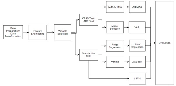
This article introduced a practical and end-to-end approach to model Point-in-Time PD in a manner that includes Forward-Looking Information for IFRS9 ECL calculation. Both traditional time series and supervised learning regression are applicable to achieve this task. Input dataset usually needs to be transformed, and new features should be created to apply learning algorithms and to achieve better performance. The variable selection process, including both quantitative and qualitative methods, should be applied in model development to have a fruitful set of predictors. The final set of selected predictors serves as the inputs to algorithms such as ARIMAX, VAR, OLS, XGBoost or LSTM, which were presented in this article. Knowing the characteristics and mechanisms of each of these algorithms can be helpful in choosing appropriate algorithms for a specific problem. Walk-Forward Validation and regression evaluation metrics (RMSE, MSE, MAE) are available to assess the performance of candidate models. Different techniques may produce results of varying accuracy depending on a specific dataset. The ‘best’ model should be selected by accessing different evaluation metrics and other aspects, e.g. related to model sensitivity.
Finalyse InsuranceFinalyse offers specialized consulting for insurance and pension sectors, focusing on risk management, actuarial modeling, and regulatory compliance. Their services include Solvency II support, IFRS 17 implementation, and climate risk assessments, ensuring robust frameworks and regulatory alignment for institutions. |

Check out Finalyse Insurance services list that could help your business.
Get to know the people behind our services, feel free to ask them any questions.
Read Finalyse client cases regarding our insurance service offer.
Read Finalyse blog articles regarding our insurance service offer.
Designed to meet regulatory and strategic requirements of the Actuarial and Risk department
Designed to meet regulatory and strategic requirements of the Actuarial and Risk department.
Designed to provide cost-efficient and independent assurance to insurance and reinsurance undertakings
Finalyse BankingFinalyse leverages 35+ years of banking expertise to guide you through regulatory challenges with tailored risk solutions. |

Designed to help your Risk Management (Validation/AI Team) department in complying with EU AI Act regulatory requirements
A tool for banks to validate the implementation of RWA calculations and be better prepared for CRR3 in 2025
In 2027, FRTB will become the European norm for Pillar I market risk. Enhanced reporting requirements will also kick in at the start of the year. Are you on track?
Finalyse ValuationValuing complex products is both costly and demanding, requiring quality data, advanced models, and expert support. Finalyse Valuation Services are tailored to client needs, ensuring transparency and ongoing collaboration. Our experts analyse and reconcile counterparty prices to explain and document any differences. |

Helping clients to reconcile price disputes
Save time reviewing the reports instead of producing them yourself
Helping institutions to cope with reporting-related requirements
Be confident about your derivative values with holistic market data at hand
Finalyse PublicationsDiscover Finalyse writings, written for you by our experienced consultants, read whitepapers, our RegBrief and blog articles to stay ahead of the trends in the Banking, Insurance and Managed Services world |

Finalyse’s take on risk-mitigation techniques and the regulatory requirements that they address
A regularly updated catalogue of key financial policy changes, focusing on risk management, reporting, governance, accounting, and trading
Read Finalyse whitepapers and research materials on trending subjects
About FinalyseOur aim is to support our clients incorporating changes and innovations in valuation, risk and compliance. We share the ambition to contribute to a sustainable and resilient financial system. Facing these extraordinary challenges is what drives us every day. |

Finalyse CareersUnlock your potential with Finalyse: as risk management pioneers with over 35 years of experience, we provide advisory services and empower clients in making informed decisions. Our mission is to support them in adapting to changes and innovations, contributing to a sustainable and resilient financial system. |

Get to know our diverse and multicultural teams, committed to bring new ideas
We combine growing fintech expertise, ownership, and a passion for tailored solutions to make a real impact
Discover our three business lines and the expert teams delivering smart, reliable support