

By Mahdi Ghazala , Senior Consultant
While carrying an action plan for implementing the new definition of default in the IT systems & processes, in its internal policies as well as in the internal models, every bank is highly interested in predicting the impact that the application of the new default definition would have on various aspects like:
That prediction can be achieved via a comprehensive simulation of the default under the new definition on the available historical data of the credit portfolio. Knowing the broad impact of the new definition on capital requirements, IFRS 9 models, precision is highly recommended for the sake of planning of own funds requirements.
To perform an accurate simulation on data of the new default definition few aspects must be considered, mainly:
We provide some practical tips regarding the above-mentioned aspects.
Simulating the new default definition on data at a time (t), will rely on a mix of two sources:
Ideally, it is preferable that the impact analysis is built on newly collected data. Indeed, the new rules are easier to apply on the new flows. The default definition is applied homogeneously and less data availability issues are faced. However, the time to entry in application of the new default definition is short and therefore the new observations window is not large enough to allow a representative simulation as well as accurate estimates of risk components, like PD, LGD or Cure rates.
That’s the reason why it is also necessary to rely on readjusted historical data. The latter is readjusted with a sufficient margin of conservatism, in particular where specific workarounds/proxies are applied to manage data unavailability issues like for instance the use of historical monthly snapshots due to unavailable historical daily data.
This is a significant challenge. On the one hand, certain criteria of detection of default status, especially some of the indications of Unlikeliness To Pay (UTP), turn out not to be even used by the institution and therefore very complex to rebuild retroactively on historical data due to lack of attributes in the existing IT systems / and in database that allows identifying such triggers.
For instance, the UTP indication “sale of credit obligation” due to the occasional character of such event it is possible that the institution doesn’t manage a sale of a portfolio of credit obligation in a specific IT system or store the information in a classical database. It may be a file / record prepared one time and stored somewhere. By consequence it will be challenging to identify those obligations flagged as sold. Even if we manage to do so, it is not guaranteed that all attributes necessary to calculate whether the economic loss is higher than 5% are available and/or reliable.
Another challenge is the identification of technical defaults that result from errors in IT systems or misunderstandings with clients rather than realization of credit risk. That generally comes from the fact that such events are partially/not covered by the institution operational policies and systems. The data at disposal could be not rich enough to allow retrace technical default situations on historical data.
So, what to do?
It is recommended to deal with such obstacles combining common sense and enough dose of conservatism with the support of experts.
The EBA Guidelines on the application of the default definition specify all aspects related to the application of the definition of default of an obligor.
For the institutions that decide to apply the definition of default for retail exposures at the obligor level it is required to specify detailed rules for the treatment of joint credit obligations and default contagion between exposures in their internal policies and procedures.
The construction of obligors base for your simulation is done through reshaping a given portfolio structure from a contract view portfolio into an obligor view portfolio reflecting the debtorness/co-debtorness links between contracts and debtors.
The final obligors table will aggregate at obligor level key information for simulating the new default detection, such as:
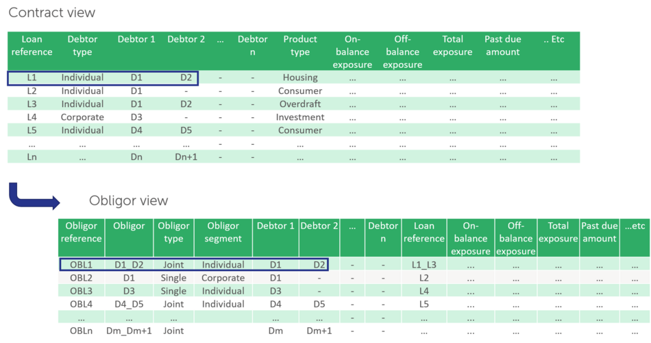
It is important that the total portfolio exposure is equal between in both views.
Additional attention points must be taken into consideration in the obligor base program, like for instance, joint-obligor segment definition or how will the obligor base be incremented/refreshed daily with new entries, or duplicates records avoidance, etc. We can help you cope with those aspects.
The obligor base program is run retro-actively on the historical daily snapshots of the portfolio that the institution has at its disposal as well as on all newly collected daily data within the defined observation horizon.
Regarding the exposure and the unpaid amount at obligor level, the calculation, at a given date, is done as follows:
This calculation is performed retro-actively on the historical daily snapshots of the portfolio that the institution has at its disposal as well as on all newly collected daily data within the defined observation horizon.
Regarding the materiality thresholds calculation and DPD counting, both are based on the information collected at a given date regarding the obligor total unpaid amount and the obligor total on-balance exposure.
Thresholds calculation
The Σ of past due amounts of all obligations linked with the obligor is >"100 EUR if Retail, 500 EUR if Non-Retail;" &
Σ of past due amounts of all obligations linked with the obligor / On-balance exposure of the obligor is > 1%. |
Days Past Due counting: The DPD counter is triggered if both conditions are met and comes back to zero if one of them stops to be met. Entry in default or exit from default status will depend on exceeding or falling below the threshold of 90 consecutive days past due. This algorithm is run retro-actively on the historical daily snapshots of the portfolio that the institution has at its disposal as well as on all newly collected daily data within the defined observation horizon. |
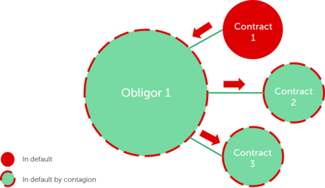
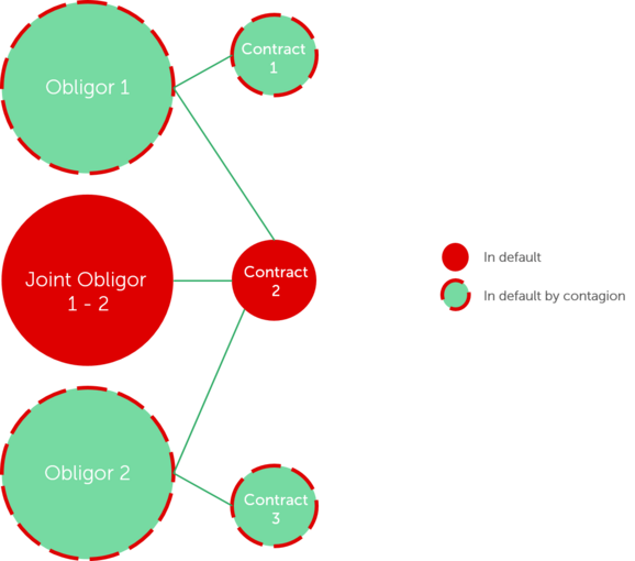
The EBA guidelines on the application of the default definition clarify important elements for the institutions applying the default for retail exposures at the obligor level. Proper understanding of those elements is important for the correct application of contagion of the default status.
In some situations, the contagion of the default status from an obligor/exposure to another is automatic. In other situations, the contagion doesn’t apply automatically and needs an additional case by case assessment. The latter is a manual individual decision difficult to simulate on data.
Below some of the situations where automatic contagion applies & therefore to be taken into consideration when simulating in the new default definition on portfolio data.
| GL 95: If any credit obligation of an obligor is in default, then all exposures to that obligor should be considered defaulted. |
| GL100: obligors with full mutual liability for an obligation, e.g. married couple where division of marital property does not apply: default of one of such obligors implies automatically the default of the other. |
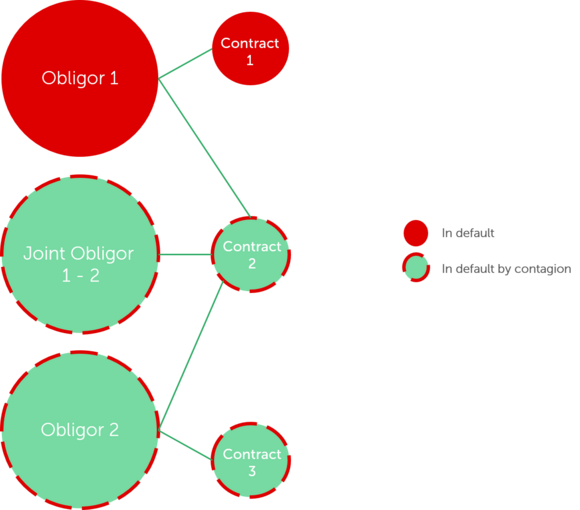
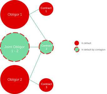
| GL97, 104: Where a joint obligor is in default, all individual obligors part of this joint obligor are automatically in default. |
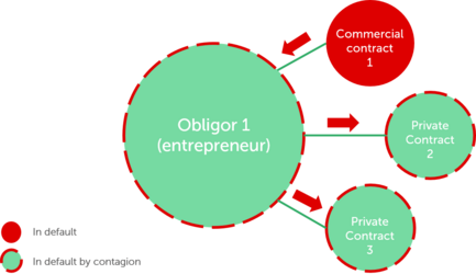
| GL102: in the specific case of an individual entrepreneur where an individual is fully liable for both private and commercial obligations, the default of any of the private or commercial obligations should cause all private and commercial obligations of such individual to be considered as defaulted as well. |
| GL 99: if all individual obligors have a defaulted status, their joint credit obligation should automatically also be considered defaulted >> the joint obligor formed by those individual obligors is automatically in default. |
As mentioned, in some situations, described in the EBA guidelines, the contagion doesn’t apply automatically but requires a case by case assessment. More details are available in the EBA Guidelines, paragraphs: 99, 100 & 105.
Now that your historical data set for the impact simulation is ready and that you have built a proper, comprehensive default detection and exit, the next step is to set the initial status (default or Sound) for all obligors/exposures of your portfolio as of the agreed initial snapshot date, that we’ll call “d”.
The goal is to obtain a first image of Performing/Non-Performing exposures/obligors based on the new definition at the date “d”.
A very important point to handle carefully is the way to manage the existing DPDs according to the old definition. There will be cases where you will reset that DPD to zero and others where you will just increment it. For that you’ll use the daily information of the last 90 days preceding “d”.
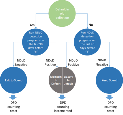
The next step will be to start from that initial date; you will run your programs to all next historical daily images of the portfolio in order to:
At the end of the exercise you qauire your evolving daily history of default/sound obligors and contracts for the whole observation period that you’ve initially fixed.
That will form the fundamental dataset you will need to perform further analysis such as transition matrix, 1year DR, impact on default portfolio in amount and number of obligors, impact on PD & LGD, cure rate, on provisions, on RWA and on capital charges. We can help you in performing such analysis.
What if you do not dispose of historical daily snapshots or not enough to perform a quantitative impact assessment?
A closer workaround solution to daily images are the monthly images. However, such should be treated with a sufficient dose of conservatism, as monthly views have several disadvantages like ignoring any entry or exit from default between two monthly snapshots due to past due or UTP.
It is important all assumptions/workaround scenarios to be approved beforehand knowing their impact on your simulation results.
A retrospective simulation of the new definition of default on data is an interesting tool for predicting the true impact of the new regulation and better anticipate any consequent capital charges. An important prerequisite to this exercise is to have a clear and correct understanding and interpretation of the rules prescribed by EBA Guidelines on the application of the default definition and by the RTS on materiality threshold of past due credit obligations.
It’s true that such exercise requires a significant effort from the bank teams in addition to the effort already engaged in implementing the new default rules in IT systems, internal policies and processes. However, this effort offers you an additional mean to assess whether new definition of default is correctly applied in the systems or not by comparing the two outputs (system based and data based); and therefore will give more comfort in validating further deployment in production.
Finalyse InsuranceFinalyse offers specialized consulting for insurance and pension sectors, focusing on risk management, actuarial modeling, and regulatory compliance. Their services include Solvency II support, IFRS 17 implementation, and climate risk assessments, ensuring robust frameworks and regulatory alignment for institutions. |

Check out Finalyse Insurance services list that could help your business.
Get to know the people behind our services, feel free to ask them any questions.
Read Finalyse client cases regarding our insurance service offer.
Read Finalyse blog articles regarding our insurance service offer.
Designed to meet regulatory and strategic requirements of the Actuarial and Risk department
Designed to meet regulatory and strategic requirements of the Actuarial and Risk department.
Designed to provide cost-efficient and independent assurance to insurance and reinsurance undertakings
Finalyse BankingFinalyse leverages 35+ years of banking expertise to guide you through regulatory challenges with tailored risk solutions. |

Designed to help your Risk Management (Validation/AI Team) department in complying with EU AI Act regulatory requirements
A tool for banks to validate the implementation of RWA calculations and be better prepared for CRR3 in 2025
In 2027, FRTB will become the European norm for Pillar I market risk. Enhanced reporting requirements will also kick in at the start of the year. Are you on track?
Finalyse ValuationValuing complex products is both costly and demanding, requiring quality data, advanced models, and expert support. Finalyse Valuation Services are tailored to client needs, ensuring transparency and ongoing collaboration. Our experts analyse and reconcile counterparty prices to explain and document any differences. |

Helping clients to reconcile price disputes
Save time reviewing the reports instead of producing them yourself
Helping institutions to cope with reporting-related requirements
Be confident about your derivative values with holistic market data at hand
Finalyse PublicationsDiscover Finalyse writings, written for you by our experienced consultants, read whitepapers, our RegBrief and blog articles to stay ahead of the trends in the Banking, Insurance and Managed Services world |

Finalyse’s take on risk-mitigation techniques and the regulatory requirements that they address
A regularly updated catalogue of key financial policy changes, focusing on risk management, reporting, governance, accounting, and trading
Read Finalyse whitepapers and research materials on trending subjects
About FinalyseOur aim is to support our clients incorporating changes and innovations in valuation, risk and compliance. We share the ambition to contribute to a sustainable and resilient financial system. Facing these extraordinary challenges is what drives us every day. |

Finalyse CareersUnlock your potential with Finalyse: as risk management pioneers with over 35 years of experience, we provide advisory services and empower clients in making informed decisions. Our mission is to support them in adapting to changes and innovations, contributing to a sustainable and resilient financial system. |

Get to know our diverse and multicultural teams, committed to bring new ideas
We combine growing fintech expertise, ownership, and a passion for tailored solutions to make a real impact
Discover our three business lines and the expert teams delivering smart, reliable support